A Four-Step Method

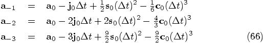
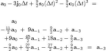
Bob: I’ll start by repeating the steps I showed you for the second-order algorithm. Instead of Eq. (46), we now have to expand the acceleration in a Taylor series up to the crackle:

And instead of Eq. (47) for the previous value of the acceleration, we now need to remember three previous values:

Alice: And these we have to invert, in order to regain the three values for , and , which we can then use in Eq. (65). The only difference is that the inversion is a little harder than it was for getting Eq. (48).

Bob: Just a little. Good luck!

Alice: Oh, I have to do it again? Well, I guess I sort-of like doing this, up to a point.

Bob: And if you dislike it, you certainly dislike it far less than I do.

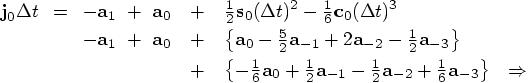
Alice: Okay, I’ll do it. From Eq. (66) we can form the following linear combination, subtracting the second equation from twice the first one, in order to eliminate the term with the jerk in it. Similarly, we can subtract the third equation from thrice the first one, and we wind up with two equations for the two remaining variables, the snap and the crackle :

Alice: Each next one will only get easier. I’ll substitute Eq. (68) in the top line of Eq. (67), and that should do it:

Alice: Now for the home run. I’ll substitute Eqs. (68) and (70) in the top line of Eq. (66), and get:

It would be much better to come up with an independent check. Ah, I see what we can do: in Eq. (66), I can check whether the solutions I just obtained for for , and indeed give us those previous three accelerations back again. In each of those three cases, I’ll start off with the right-hand sides of the equation, to see whether I’ll get the left-hand side back.

Here is the first one:

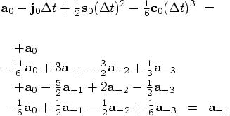
Bob: Good start!

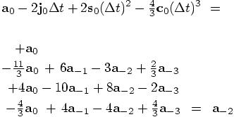
Alice: And a good middle part, too. Now for the finish:

Good! Clearly, the expressions in Eqs. (72), (70) and (68) are correct. Phew! And now that that is done . . . what was it again we set out to do?

Bob: We were trying to get an expression for the acceleration at time zero, to third order in the time step, expressed in terms of the previous three accelerations. So all we have to do is to plug your results back into Eq. (65).

Alice: Ah, yes, it’s easy to forget the thread of a story, if you get lost in eliminations.

Implementation

Bob: So now it’s my turn, I guess. Let me code up your results. I’ll open a new file, ms4body.rb. Let me first have a look at the previous second-order method ms2, for comparison:

   def ms2(dt)
     if @nsteps == 0
       @prev_acc = acc
       rk2(dt)
     else
       old_acc = acc
       jdt = old_acc - @prev_acc
       @pos += vel*dt + old_acc*0.5*dt*dt
       @vel += old_acc*dt + jdt*0.5*dt
       @prev_acc = old_acc
     end
   end

Our fourth-order multi-step method should be called ms4, clearly. I’ll use rk4 to rev up the engine, something we’ll have to do three times now. And instead of use snap and crackle out-of-the-box, so to speak, I’ll use them with the appropriate factors of the time step, and , respectively.

Here are the equations that we have to code up, as a generalization of Eq. ():

   def ms4(dt)
     if @nsteps == 0
       @ap3 = acc
       rk4(dt)
     elsif @nsteps == 1
       @ap2 = acc
       rk4(dt)
     elsif @nsteps == 2
       @ap1 = acc
       rk4(dt)
     else
       ap0 = acc
       jdt = ap0*(11.0/6.0) - @ap1*3 + @ap2*1.5 - @ap3/3.0
       sdt2 = ap0*2 - @ap1*5 + @ap2*4 - @ap3
       cdt3 = ap0 - @ap1*3 + @ap2*3 - @ap3
       @pos += vel*dt + (ap0/2.0 + jdt/6.0 + sdt2/24.0)*dt*dt
       @vel += ap0*dt + (jdt/2.0 + sdt2/6.0 + cdt3/24.0)*dt
       @ap3 = @ap2
       @ap2 = @ap1
       @ap1 = ap0
     end
   end

Alice: That’s not so much longer than ms2, and it still looks neat and orderly! And wait, you have used the division method for our Vector class, in dividing by those number like and so on.

Bob: That’s true! I hadn’t even thought about it; it was so natural to do that. What did you say again, when I told you I had added division, together with subtraction, to the Vector class?

Alice: I said that I was sure it would come in handy sooner or later.

Bob: I guess it was sooner rather than later.

Alice: And I see that you have abbreviated the names of the variables somewhat. Instead of @prev_acc for the previous acceleration, you now use @ap1, for the first previous acceleration, I guess. And then, for the yet more previous acceleration before that, you use @ap2, and so on.

Bob: Yes. I would have like to write a-2 for but that would be interpreted as a subtraction of the number 2 from the variable a, so I choose @ap2, for a-previous-two.

Testing

 |gravity> ruby integrator_driver4d.rb < euler.in
 dt = 0.01
 dt_dia = 0.1
 dt_out = 0.1
 dt_end = 0.1
 method = ms4
 at time t = 0, after 0 steps :
   E_kin = 0.125 , E_pot =  -1 , E_tot = -0.875
              E_tot - E_init = 0
   (E_tot - E_init) / E_init =-0
 at time t = 0.1, after 10 steps :
   E_kin = 0.129 , E_pot =  -1 , E_tot = -0.875
              E_tot - E_init = 1.29e-10
   (E_tot - E_init) / E_init =-1.48e-10
   1.0000000000000000e+00
   9.9499478015881193e-01  4.9916426246428156e-02
  -1.0020902652762116e-01  4.9748796059474770e-01

 |gravity> ruby integrator_driver4e.rb < euler.in
 dt = 0.001
 dt_dia = 0.1
 dt_out = 0.1
 dt_end = 0.1
 method = ms4
 at time t = 0, after 0 steps :
   E_kin = 0.125 , E_pot =  -1 , E_tot = -0.875
              E_tot - E_init = 0
   (E_tot - E_init) / E_init =-0
 at time t = 0.1, after 100 steps :
   E_kin = 0.129 , E_pot =  -1 , E_tot = -0.875
              E_tot - E_init = 2.24e-14
   (E_tot - E_init) / E_init =-2.56e-14
   1.0000000000000000e+00
   9.9499478008957187e-01  4.9916426216151437e-02
  -1.0020902860087451e-01  4.9748796006061335e-01

 |gravity> ruby integrator_driver4f.rb < euler.in
 dt = 0.002
 dt_dia = 0.1
 dt_out = 0.1
 dt_end = 0.1
 method = ms4
 at time t = 0, after 0 steps :
   E_kin = 0.125 , E_pot =  -1 , E_tot = -0.875
              E_tot - E_init = 0
   (E_tot - E_init) / E_init =-0
 at time t = 0.1, after 50 steps :
   E_kin = 0.129 , E_pot =  -1 , E_tot = -0.875
              E_tot - E_init = 3.45e-13
   (E_tot - E_init) / E_init =-3.95e-13
   1.0000000000000000e+00
   9.9499478008976872e-01  4.9916426216220194e-02
  -1.0020902859668304e-01  4.9748796006170143e-01

Alice: Given that I already reconstructed your instructions on paper before, I only have to extend it to two orders higher. Here are the results on a backward extrapolation, starting with the predicted values at time , and going back to time , as a higher-order analogy of Eq. (53) :

where again 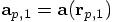and where , , and are the jerk, snap, and crackle as determined from the values of the last four accelerations, which are now 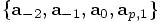, instead of the previous series of four that were used in the prediction step, which were .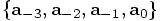

The same arguments as I gave before will now lead to the following expression for the first-iteration solution for the corrected quantities, as an extension of Eq. (61)

Note that once more I have interchanged the order of the calculations of the position and velocity: by calculating the corrected value of the velocity first, I am able to use that one in the expression for the corrected value of the position.

Bob: And this time I certainly do not recognize these equations. It seems that we really have a new algorithm here.

Alice: Let me see whether I can extend your code, to implement this scheme. It would be nice to keep the number of acceleration calculations the same as we had before, doing it only once per time step. After all, when we will generalize this to a true N-body system, it is the calculation of the acceleration that will be most expensive, given that for each particle we will have to loop over all other particles.

However, I need to compute the acceleration at the end of the calculation, at the newly predicted position. This means that I then have to remember the value of the acceleration, so that I could reuse it at the beginning of the next time step. This means that I will have to change the variable ap0 to a true instance variable @ap0, so that it will still be there, the next time we enter ms4pc.

I will have to initialize @ap0 during the last time we use the rk4 method, so that it is ready to be used when we finally enter the main body of the ms4pc method, as I will call it, to distinguish it from your previous implementation ms4.

Bob: The pc stands for predictor-corrector version, I take it.

Implementation

   def ms4pc(dt)
     if @nsteps == 0
       @ap3 = acc
       rk4(dt)
     elsif @nsteps == 1
       @ap2 = acc
       rk4(dt)
     elsif @nsteps == 2
       @ap1 = acc
       rk4(dt)
       @ap0 = acc
     else
       old_pos = pos
       old_vel = vel
       jdt = @ap0*(11.0/6.0) - @ap1*3 + @ap2*1.5 - @ap3/3.0
       sdt2 = @ap0*2 - @ap1*5 + @ap2*4 - @ap3
       cdt3 = @ap0 - @ap1*3 + @ap2*3 - @ap3
       @pos += vel*dt + (@ap0/2.0 + jdt/6.0 + sdt2/24.0)*dt*dt
       @ap3 = @ap2
       @ap2 = @ap1
       @ap1 = @ap0
       @ap0 = acc
       jdt = @ap0*(11.0/6.0) - @ap1*3 + @ap2*1.5 - @ap3/3.0
       sdt2 = @ap0*2 - @ap1*5 + @ap2*4 - @ap3
       cdt3 = @ap0 - @ap1*3 + @ap2*3 - @ap3
       @vel = old_vel + @ap0*dt + (-jdt/2.0 + sdt2/6.0 - cdt3/24.0)*dt
       @pos = old_pos + vel*dt + (-@ap0/2.0 + jdt/6.0 - sdt2/24.0)*dt*dt
     end
   end

 |gravity> ruby integrator_driver4dpc_old.rb < euler.in
 dt = 0.01
 dt_dia = 0.1
 dt_out = 0.1
 dt_end = 0.1
 method = ms4pc
 at time t = 0, after 0 steps :
   E_kin = 0.125 , E_pot =  -1 , E_tot = -0.875
              E_tot - E_init = 0
   (E_tot - E_init) / E_init =-0
 ./ms4body_old.rb:158:in `ms4pc': undefined method `-@' for [-0.000500866850078996, -0.00502304344952675]:Vector (NoMethodError)
        from ./ms4body_old.rb:22:in `send'
        from ./ms4body_old.rb:22:in `evolve'
        from integrator_driver4dpc_old.rb:21

Bob: Beats me. I know what the method - is, that is just the subtraction method, which I have neatly defined for our Vector class, while I was implementing the second-order version of our series of multi-step integrators. I have no idea as to what the method -@ could possibly be.

But let us look at the code first, maybe that will tell us something. I’ll scrutinize all the minus signs, to see whether we can find a clue there. The middle part of the method ms4pc is the same as in the predictor-only method ms4, and that one did not give any errors. So we’ll have to look in the last five lines. The first three of those are verbatim copies of the lines above, which were already tested, we the culprit really should lurk somewhere in the last two lines.

Hmm, minus sign, last two lines, ahaha! Unary minus!!

Alice: Unary minus?? As opposed to a dualistic minus?

Bob: As opposed to a binary minus. There are two different meanings of a minus sign, logically speaking: the minus in and the minus in . In the first example, the minus indicates that you are subtracting two numbers. You could write that operation as . In the second example, you are dealing only with one number, and you take the negative value of that number. You could write that as .

So in the first case, you have a binary operator, with two arguments, and in the second case, you have a unary operator, with only one argument. Hence the name `unary minus.’

Alice: A binary minus, hey? I’m getting more and more confused with all those different things that are called binaries. In astronomy we call double stars binaries, in computer science they use binary trees in data structures, and binary notation for the ones and zeros in a register, and we talk about binary data as opposed to ASCII data, and now even a lowly minus can become a binary. Oh well, I guess each use has its own logic.

Bob: And many things in the universe come in pairs.

Alice: Even people trying to write a toy model and stumbling upon unary minuses — or unary mini? Anyway, I see now that the minus sign that I added in front of the jerk in the middle of the line

       @vel = old_vel + @ap0*dt + (-jdt/2.0 + sdt2/6.0 - cdt3/24.0)*dt

was a unary minus. All very logical. And yes, while we had defined a binary minus before, we had not yet defined a unary minus.

Bob: So you committed a logopo.

Alice: And I could correct my logopo by writing jdt/(-2.0) instead of -jdt/2.0. However, I don’t like to do that, it looks quite ugly.

Bob: The alternative is to add a unary minus to our Vector class.

Alice: I would like that much better! How do you do that?

Bob: Judging from the error message, Ruby seems to use the convention that -@ stands for unary minus. But just to make sure, let me look at the manual. Just a moment . . .

. . . and yes, my interpretation was correct. So let’s just add it to our collections of methods in the file vector.rb. How about the following extension, within the Vector class:

   def -@
     self.map{|x| -x}.to_v
   end

and for good measure, I may as well add a unary plus too:

   def +@
     self
   end

Alice: I see, just in case you write something like r_new = +r_old.

Bob: Exactly. No need to do so, but also no need to let that give you an error message if you do.

Testing

 |gravity> ruby integrator_driver4dpc.rb < euler.in
 dt = 0.01
 dt_dia = 0.1
 dt_out = 0.1
 dt_end = 0.1
 method = ms4pc
 at time t = 0, after 0 steps :
   E_kin = 0.125 , E_pot =  -1 , E_tot = -0.875
              E_tot - E_init = 0
   (E_tot - E_init) / E_init =-0
 at time t = 0.1, after 10 steps :
   E_kin = 0.129 , E_pot =  -1 , E_tot = -0.875
              E_tot - E_init = -9.56e-12
   (E_tot - E_init) / E_init =1.09e-11
   1.0000000000000000e+00
   9.9499478008669873e-01  4.9916426232219237e-02
  -1.0020902876280345e-01  4.9748796001291246e-01

 |gravity> ruby integrator_driver4epc.rb < euler.in
 dt = 0.001
 dt_dia = 0.1
 dt_out = 0.1
 dt_end = 0.1
 method = ms4pc
 at time t = 0, after 0 steps :
   E_kin = 0.125 , E_pot =  -1 , E_tot = -0.875
              E_tot - E_init = 0
   (E_tot - E_init) / E_init =-0
 at time t = 0.1, after 100 steps :
   E_kin = 0.129 , E_pot =  -1 , E_tot = -0.875
              E_tot - E_init = -1.11e-15
   (E_tot - E_init) / E_init =1.27e-15
   1.0000000000000000e+00
   9.9499478008955766e-01  4.9916426216148800e-02
  -1.0020902860118561e-01  4.9748796006053242e-01