Orbit vs. Interaction
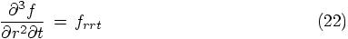
Space and Time Dependent Interactions
Bob: So you claim that our somewhat tedious proof isn’t ironclad yet? You said something about having checked time variations but not space variations. Could you explain that in a bit more detail? I’m afraid I didn’t quite get it.
Alice: I’m still grappling with it myself. This stuff is not easy. No wonder people can spend a life time on designing numerical methods. Linear and quadratic methods are not too hard, since you can still sketch on a piece of paper what is going on. But by the time you’re dealing with a fourth-order or higher method, you can no longer use your intuition. And when you switch to formal proofs, it is easy to overlook things. I’m sure we’ve done just that, but let me see whether I can really put my finger on it.
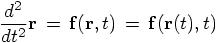
What I meant was that any differential equation in a dynamical system has a left-hand side that tells us how the orbit of a particle changes in time as a result of interactions with the rest of the world. The dynamics is specified on the right-hand side, while the left-hand side shows only the kinematics. In other words, the physical forces can be found on the right-hand side, while the mathematical description of the deflection of the orbit, as a result of those forces, is given on the left-hand side.
Bob: I find it always easier to look at a specific example. Here we have our Newtonian equations of motion, for the gravitational two-body problem.
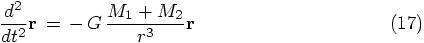
Indeed, the physical coupling constant G appears only on the right-hand side, where the gravitational interaction is specified, while the left-hand side tells us how the orbit is bent: non-zero acceleration describes the deviation of uniform rectilinear motion. Okay, I’m still with you.
Alice: Now the trick is to make explicit what we normal vaguely understand, but rarely write down precisely, namely the space and time dependence of the interaction. In any N-body system, whether we have two particles or a million, each particle feels a time-varying force field.
Bob: And that is what makes it non-trivial to do an N-body simulation. If we only had to integrate the orbit of a particle rolling through a fixed potential landscape, life would be a lot easier. The problem is that everything changes all the time: one moment a particle is coasting along happily, and before you know it, suddenly it crosses the orbit of another particle, resulting is a sharp deflection.
Alice: So let’s write that down in a general way, not worrying about any details of the actual interaction, but just making clear that the interaction is both space and time dependent:
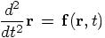
Bob: Meaning that on the left you have the acceleration and on the right you have the force.
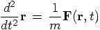
Alice: Not quite: if we denote the actual force by  , we should write:
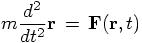
which for the acceleration would give
where  is the mass of the
particle; or in the case of two-body motion, the reduced mass associated
with the motion of the equivalent one-body system, for a pseudo-particle in
a time varying force field.
is the mass of the
particle; or in the case of two-body motion, the reduced mass associated
with the motion of the equivalent one-body system, for a pseudo-particle in
a time varying force field.
Anyway, those details are irrelevant here. My point is that I prefer to talk about orbit vs. interaction, not orbit vs. force calculation.
Bob: In stellar dynamics, at least, people talk about force calculation all the time.
Alice: I know, and then they write down the acceleration. We‘ve seen already how easy it is to get into trouble when forgetting to take the mass into account properly.
Bob: Well, yes, I can’t argue with that, I’m afraid, seeing how I blundered there, a while ago.
Alice: So let us call  the general interaction term that causes an
acceleration to occur. That is in line with the notation in books about
general differential equations. Abramowitz and Stegun used the same
notation too.
the general interaction term that causes an
acceleration to occur. That is in line with the notation in books about
general differential equations. Abramowitz and Stegun used the same
notation too.
The One-Dimensional Case
Bob: Now that we have settled nomenclature, can we look at what you claimed went wrong with our derivation?
Alice: My point is that we have to be really explicit about the space and time dependence of the interaction terms, as follows:
Bob: This is what we did. We considered the time dependence of the orbit, and how that fed back into the time dependence of the interaction term.
Alice: Yes, and we looked at the error term in terms of time dependence. But we did not check the other contribution to the error in the position, stemming from the fact that our orbit makes errors in space as well as in time.
Eq. (8) for  , for example, is written in terms of
orbit variables, using only concepts from the left-hand side of
the differential equations that we are trying to solve. But if you look at
your code, just above that equation, you see that the term a2 in
your code is a call to the method acc, which does an
interaction calculation: it invokes the right-hand side of the
differential equation.
, for example, is written in terms of
orbit variables, using only concepts from the left-hand side of
the differential equations that we are trying to solve. But if you look at
your code, just above that equation, you see that the term a2 in
your code is a call to the method acc, which does an
interaction calculation: it invokes the right-hand side of the
differential equation.
Bob: I guess that that was not quite consistent. How do you propose to remedy our analysis?
Alice: If we really wanted to be formally correct, we could track the four-dimensional variations in space and time, taking into account the three-dimensional spatial gradient of the interaction terms.
Bob: But from the way you just said that, I figure that that would be too much, even for you. I’m glad to hear that even you have your limits in wanting to check things analytically!
Alice: I sure have. And also, I don’t think such a formal treatment would be necessary. If we can prove things in one dimension, I’m convinced that we could rewrite our prove to three dimensions without too many problems, albeit with a lot more manipulations.
Bob: You won’t hear me arguing against simplification! But I must admit, you have made me curious. Go on!
Alice: What I propose is that we go back to the way Abramowitz and Stegun formulated their Runge-Kutta version. After all, the whole discussion was about whether their claim of having a fourth-order error was a misprint or not. If we can prove that their method, as they stated it, is fourth-order accurate, with an error that scales like the fifth power of the time step, I’m satisfied.
A Change in Notation
Bob: Same for me. But I propose that we use a somewhat more intuitive notation than what they gave us. To use x to indicate time and y to indicate position is confusing, to say the least. Let us look at the text again:

How about the following translation, where the position r, velocity v, and a are all scalar quantities, since we are considering an effectively one-dimensional problem:
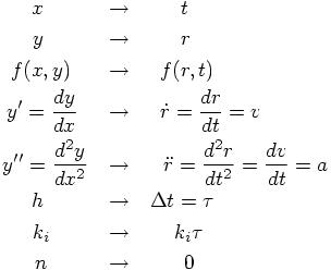
The equations, as proposed by Abramowitz and Stegun, then become:
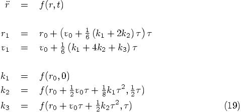
The Auxiliary k Variables
Alice: Yes, I find that notation much more congenial, and I’m glad to see the explicitly space and time dependence now in the definitions of the three k variables.
Let us work out what these k variables actually look like, when we
substitute the orbit dependence in the right hand side. What we see there
is an interesting interplay between a physical interaction term f
that has as an argument the mathematical orbit  .
.
Since you have introduced  as the increment in time, starting from time
zero, let me introduce the variable
as the increment in time, starting from time
zero, let me introduce the variable  to indicate the increment in space, the
increment in position at the time that we evaluate
to indicate the increment in space, the
increment in position at the time that we evaluate 

For consistency, let me also use

for the increment in time, when we evaluate  . Let me also abbreviate
 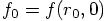 .
.
What I propose to do now is to expand  in a double Taylor series, simultaneously in
space and in time. This will hopefully repair the oversight we made before,
when we only considered a time expansion.
in a double Taylor series, simultaneously in
space and in time. This will hopefully repair the oversight we made before,
when we only considered a time expansion.
Bob: How do you do a two-dimensional Taylor series expansion?
Alice: Whenever you have mixed derivatives, such as
you multiply the coefficients you would give to each dimension separately; in this case you would get a factor of one half, because of the second partial derivative with respect to space; the single time derivative just gives a factor one. You can easily check how this work when you look at a two-dimensional landscape, and you imagine how you pick up difference in height by moving North-South and East-West. Anyway, here is the concrete example, for our case, where I use the abbreviation that I introduced above, with partial differentiation indicated with subscripts:
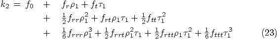
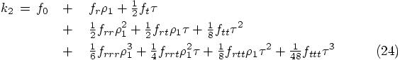
where I have grouped the different orders of expansion in terms of small
variables on different lines. Using the fact that  , we can also write this as
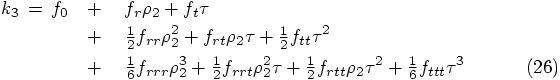
Similarly, we can introduce

as the spatial offset in the argument for the interaction term for the
calculation of  , for
which we get:
, for
which we get:
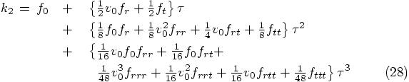
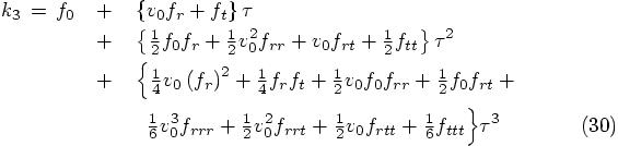
Now the next step is to substitute the definitions of the  variables in the
  equations, and to keep terms
up to the third order in
equations, and to keep terms
up to the third order in  .
.
The Next Position
Bob: That’s going to be quite messy.
Alice: Well, yes, but we have no choice. Let me start with the
substitution indicated in Eq. (20), where we may as well
replace  by its value
 :
:

which is just its Taylor series expansion in time, up to second order. Using this substitution in Eq. (24), we get:
Similarly, we have to take Eq. (26), where we have to use
the substitution indicated in Eq. (25), which we can
rewrite, using the expression for  that we just derived, up till third order in
 , as;
, as;

Bob: And now I see concretely what you meant, when you said that our
previous attempt at proving the fourth-order nature of the Runge-Kutta
integrator neglected the treatment of the right-hand side of the
differential equation, of the physical interaction terms. They would not
have showed up if we were trying to prove the correctness of a second-order
Runge-Kutta scheme. It is only at third order in  that they appear, in the form of partial
derivatives of the interaction term.
that they appear, in the form of partial
derivatives of the interaction term.
Alice: Yes, that must be right. Okay, ready for a next round of substitution? Eq. (26) then becomes:
We are now in a position to evaluate the solution that our Runge-Kutta
scheme gives us for the value of the position and velocity in the next time
step, as given in Eq. (19), since there we can now
substitute  and
and  in the expressions for
  and
and  .
.
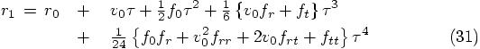
Starting with the position, we find:
The Next Velocity
Bob: And the last term in curly brackets, in the first line of the last equation must be the jerk. I begin to see some structure in these expressions.
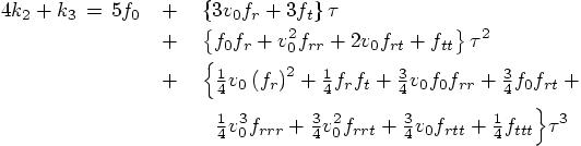
Alice: Yes. But let me get the velocity as well, and then we can
take stock of the whole situation. Let’s see. To solve for  in Eq. (19), we need to use the following combination of
  values:
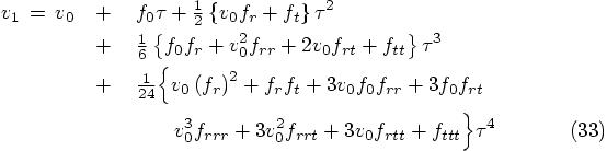
Plugging this back into the expression for  in Eq. (19), we get:
Bob: Quite an expression. Well done!
Alice: And an expression that makes sense: we see that indeed the velocity, Eq. (33), is the time derivative of the position, Eq. (31), up to the order given there. So everything is consistent.
Everything Falls into Place
Bob: So where do we stand now? This was all nice and fine, but I must admit, I’m beginning to lose the forest for the trees.
Alice: What we have done now is to compute the predicted positions and velocities after one time step, and we have checked that if we vary the length of the time step, we indeed find that the velocity changes like the time derivative of the position. The question is: are they really solutions of the equations of motion that we started out with, up to the fourth order in the time step size?
Let us go back to the equations of motion, in the form we gave them just after we translated the expressions from Abramowitz and Stegun:

For time zero this gives:

We can differentiate the equation for  , to find the jerk:

which gives us at the starting time:

When we differentiate the equation for  , we find the snap:

or at time  :
:

Next, with one more differentiation of the equation for  , we can derive the crackle:

Using the expression for the jerk, that we found above, we find for time zero:

Bob: I see, now the clouds are clearing, and the sun is shining through! When you substitute these values back into the equation for the new position, Eq. (31), we find:

and similarly, for Eq. (33), we find:

Both are nothing else but the Taylor series for their orbits.
Alice: And now we have derived them in a fully space-time dependent way.
Bob: Congratulations! I’m certainly happy with this result. But I must admit, I do wonder whether this conclusion would satisfy a mathematician working in numerical analysis.
Alice: Probably not. Actually, I hope not. I’m glad some people are more careful than we are, to make sure that our algorithms really do what we hope they do. At the same time, I’m sure enough now that we have a reasonable understanding of what is going on, and I’m ready to move on.
Bob: I certainly wouldn’t ask my students to delve deeper into this matter than we have been doing so far. At some point they will have to get results from their simulations.
Alice: At the same time, unless they have a fair amount of understanding of the algorithms that they rely on, it will be easy for them to use those algorithms in the wrong way, or in circumstances where their use is not appropriate. But I agree, too much of a good thing may simply be too much. Still, if a student would come to be with a burning curiosity to find out more about what is really going on with these higher-order integration methods, I would encourage that him or her to get deeper into the matter, through books or papers in numerical analysis.
Bob: I don’t think that is too likely to happen, but if such students appear on my doorsteps, I’m happy to send them to you!
Alice: And I would be happy too, since I might well learn from them. I’ve the feeling that we’ve only scratched the surface so far.
Debugging All and Everything?
Bob: Yes, and our scratching had some hits and some misses. If we are ever going to write up all this exploring we are doing now, for the benefit of our students, we have to decide what to tell them, and what to sweep under the rug.
Alice: I suggest we tell them everything, the whole story of how and where we went wrong. If we’re going to clean up everything, we will wind up with a text book, and text books there are already enough of in this world.
Bob: I wasn’t thinking about any formal publication, good grief, that would be far too much work! I was only thinking about handing out notes to the students in my class. And I must say, I like the idea of showing them a look into our kitchen. I think it will be much more interesting for the students, and after all, if you and I are making these kinds of mistakes, we can’t very well pretend that the students would be above making those types of mistakes, can we?
Alice: Precisely. They may learn from our example, in two ways: they will realize that everyone makes mistakes all the time, and that every mistake is a good opportunity to learn more about the situation at hand. Debugging is not only something you have to do with computer programs. When doing analytical work, you also have to debug both the equations you write down, in which you will make mistake, as well as the understanding you bring to the writing down in the first place.
You might even want to go so far as to say that life is one large debugging process. I heard Gerald Sussman saying something like that, some day. He was in a talkative mood, as usual. Somebody asked him what he meant when he said that he considers himself to be a philosophical engineer, and that was his answer.
Bob: I doubt that I will have to debug my beer, I sure hope not! But as far as codes and math and physics, sure, I’d buy that. So yes, let us present the students our temporary failures on the level of math as well as on the level of coding. I’m all for it!
Alice: So, what’s next? A sixth order integrator?
Bob: I hadn’t thought about that, but given the speed-up we got with going from rk2 to rk4, it would be interesting to see whether this happy process will continue when we would go to a rk6 method, for a sixth-order Runge-Kutta method. The problem is that Abramowitz and Stegun don’t go beyond fourth order methods. Hmm. I’ll look around, and see what I can find.