Runge Kutta

Two New Integrators

Alice: Good morning, Bob! Any luck with extending your menu of integrators?

Bob: Yes, I added two Runge-Kutta integrators, one second-order and one fourth-order in accuracy. The changes are again minimal.

For the driver program there is no change at all. The only difference is that you can now call evolve with method = "rk2" to invoke the second-order Runge-Kutta integrator, or "rk4" for the fourth-order integrator.

Bob: The Runge-Kutta method does not leap, as the leapfrog does. It is more careful. It feels its way forward by a half-step, sniffs out the situation, returns again, and only then it makes a full step, using the information gained in the half-step.

Alice: Like a cat?

Bob: Do cats move that way?

Alice: Sometimes, when they are trying to catch a mouse, they behave as if they haven’t seen their prey at all. They just meander a bit, and then return, so that the poor animal thinks that it is safe now. But then, when the mouse comes out of hiding, the cat pounces.

Bob: So we should call the Runge-Kutta method the leapcat method?

Alice: Why not?

Bob: I’m not sure. For one thing, my code doesn’t meander. You can tell your students what you like, I think I’ll be conservative and stick to Runge Kutta.

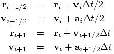
Here are the equations that incorporate the idea of making a half-step first as a feeler:

Alice: Ah yes, now it is very clear how you use the information from the half-step, in the form of the velocity and acceleration there, to improve the accuracy of the full step you take at the end.

Bob: Wait a minute. Looking again at the equations that I got from a book yesterday, I begin to wonder. Is this really different from the leapfrog method? We have seen that you can write the leapfrog in at least two quite different ways. Perhaps this is a third way to write it?

Alice: I think it is different, otherwise it would not have a different name, but it is a good idea to check for ourselves. Let us write out the effect of the equations above, by writing the half-step values in terms of the original values. First, let’s do it for the position:

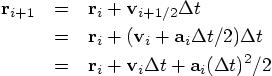
Bob: Hey, that is the exact same equation as we had for the leapfrog. Now I’m curious what the velocity equation will tell us.

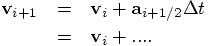
Ah, that doesn’t work, we cannot write in terms of quantities at times and . It really is a new result, computed halfway.

Alice: You are right. So the two methods are really different then. Good to know. Still, let us see how different they are. The corresponding equation for the leapfrog is:

Bob: Ah, that is neat. The Leapfrog velocity jump uses the average acceleration, averaged between the values at the beginning and at the end of the leap. The Runge-Kutta method approximates this average by taking the midpoint value.

Alice: Or putting it the other way around, the leapfrog approximates the midpoint value by taking the average of the two accelerations.

Bob: Yes, you can look at it both ways. In fact, if you take your view, you can see that the leapfrog is twice as efficient as Runge-Kutta, in that it calculates only the accelerations at the integer time points. In contrast, the Runge-Kutta method also calculates the accelerations at the half-integer points in time. So it requires twice as many acceleration calculations.

Of course, in my current code that is not obvious, since I am calculating the acceleration twice in the leapfrog as well. However, it would be easy to rewrite it in such a way that it needs only once acceleration calculation. And in the Runge-Kutta method you cannot do that.

Translating Formulas Again

Alice: Going back to the original equations you wrote down for your second-order Runge-Kutta code:

I must admit that your way of coding them up is not immediately transparent to me. If I had to implement these equations, I would have written something like:

  def rk2(dt)
    old_pos = pos
    old_vel = vel
    half_pos = pos + vel*0.5*dt
    half_vel = vel + acc*0.5*dt
    @pos = half_pos
    half_acc = acc
    @vel = old_vel + half_acc*dt
    @pos = old_pos + half_vel*dt
  end

Bob: Yes, that is how I started as well. But then I realized that I could save three lines by writing them the way I did in the code:

   def rk2(dt)
     old_pos = pos
     half_vel = vel + acc*0.5*dt
     @pos += vel*0.5*dt
     @vel += acc*dt
     @pos = old_pos + half_vel*dt
   end

The number of times you calculate the acceleration is the same, but instead of introducing five new variable, I only introduced two.

Alice: it is probably a good idea to show both ways to the students, so that the whole process of coding up an algorithm becomes more transparent to them.

Bob: Yes, I’ll make sure to mention that to them.

Energy Conservation

Alice: Since we know now that the two methods are different, it seems likely that the energy conservation in the Runge-Kutta method is a better indicator for the magnitude of the positional errors than it was in the leapfrog case. Shall we try the same values as we used before, but now for the Runge-Kutta method?

Bob: Sure. But before doing that, note that the position error in our first run is about , where we had for the leapfrog. So the Runge-Kutta, for a time step of 0.001, is a hundred times worse in energy conservation and ten times worse in the accuracy of the positions, compared with the leapfrog. Then, at a time step of 0.0001, the energy error lags only a factor ten behind the leapfrog. Okay, let’s go to a time step of 0.00001:

 |gravity> ruby integrator_driver2c.rb < euler.in
 dt = 1.0e-05
 dt_dia = 10
 dt_out = 10
 dt_end = 10
 method = rk2
 at time t = 0, after 0 steps :
   E_kin = 0.125 , E_pot =  -1 , E_tot = -0.875
              E_tot - E_init = 0
   (E_tot - E_init) / E_init =-0
 at time t = 10, after 1000000 steps :
   E_kin = 0.554 , E_pot =  -1.43 , E_tot = -0.875
              E_tot - E_init = 6.41e-11
   (E_tot - E_init) / E_init =-7.32e-11
   1.0000000000000000e+00
   5.9961749187967806e-01 -3.6063469285477523e-01
   1.0308069441700245e+00  2.1389511823566043e-01

Alice: The third-order style behavior continues! The energy error again shrunk by a factor a thousand. Now the leapfrog and Runge-Kutta are comparable in energy error, to within a factor of two or so.

Bob: The position error of our second run was , as we can now see by comparison with the third run. That is strange. The positional accuracy increases by a factor 100, yet the energy accuracy increases by a factor 1000.

Alice: Let’s shrink the step size by another factor of ten.

    |gravity> ruby integrator_driver2.rb < euler.in
    dt = 1.0e-06
    dt_dia = 10
    dt_out = 10
    dt_end = 10
    method = rk2
    at time t = 0, after 0 steps :
      E_kin = 0.125 , E_pot =  -1, E_tot = -0.875
                 E_tot - E_init = 0
      (E_tot - E_init) / E_init =-0
    at time t = 10, after 10000000 steps :
      E_kin = 0.554 , E_pot =  -1.43, E_tot = -0.875
                 E_tot - E_init = -1.66e-13
      (E_tot - E_init) / E_init =1.9e-13
      1.0000000000000000e+00
      5.9961755426085783e-01 -3.6063458453782676e-01
      1.0308069106006272e+00  2.1389530234024676e-01

Bob: This time the energy error shrunk only by two and a half orders of magnitude, about a factor 300, but still more than the factor hundred than we would have expected. Also, with integration steps, I’m surprised we got even that far. At each time, round off errors must occur in the calculations that are of order . Then statistical noise in so many calculations must be larger than that by at least the square root of the number of time steps, or .

Alice: Which is close to what we got. So that would suggest that further shrinking the time step would not give us more accuracy.

Bob: I would expect so much. But these calculations are taking a long time again, so I’ll let the computer start the calculation, and we can check later. At least now we are pushing machine accuracy for 64-bit floating point with our second-order integrator; a while ago it took forever to get the errors in position down to one percent. I can’t wait to show you my fourth-order integrator. That will go a lot faster. But first let’s see what we get here.

. . . . .

Reaching the Round-Off Barrier

Alice: It has been quite a while now. Surely the code must have run now.

Bob: Indeed, here are the results.

    |gravity> ruby integrator_driver2.rb < euler.in
    dt = 1.0e-07
    dt_dia = 10
    dt_out = 10
    dt_end = 10
    method = rk2
    at time t = 0, after 0 steps :
      E_kin = 0.125 , E_pot =  -1, E_tot = -0.875
                 E_tot - E_init = 0
      (E_tot - E_init) / E_init =-0
    at time t = 10, after 100000000 steps :
      E_kin = 0.554 , E_pot =  -1.43, E_tot = -0.875
                 E_tot - E_init = -4.77e-13
      (E_tot - E_init) / E_init =5.45e-13
      1.0000000000000000e+00
      5.9961755488235224e-01 -3.6063458345517674e-01
      1.0308069102692998e+00  2.1389530417820268e-01

As we expected, the energy error could not shrink further. Instead, it grew larger, because the random accumulation of errors in ten times more time steps gave an increase of error by roughly the square root of ten, or about a factor three — just what we observe here.

Alice: Note that the positions now agree to within a factor of . Once more a factor a hundred more accurate than the difference between the previous two integrations. Clearly the positional accuracy of the second order Runge-Kutta is second-order accurate, like that of the leapfrog.