Leapfrog
The Basic Equations
Alice: Hi, Bob! Any luck in getting a second order integrator to work?
Bob: No problem, it was easy! Actually, I got two different ones to work, and a fourth order integrator as well.
Alice: Wow, that was more than I expected!
Bob: Let’s start with the second order leapfrog integrator.
Alice: Wait, I know what a leapfrog is, but we’d better make some notes about how to present the idea to your students. How can we do that quickly?
Bob: Let me give it a try. The name leapfrog comes from one
of the ways to write this algorithm, where positions and velocities `leap
over’ each other. Positions are defined at times 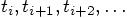 , spaced at constant intervals
  , while the velocities are
defined at times halfway in between, indicated by
, while the velocities are
defined at times halfway in between, indicated by 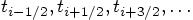 , where
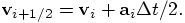
  . The leapfrog integration scheme then reads:
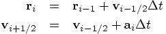
Note that the accelerations  are defined only on integer times, just like
the positions, while the velocities are defined only on half-integer times.
This makes sense, given that
are defined only on integer times, just like
the positions, while the velocities are defined only on half-integer times.
This makes sense, given that 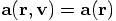 : the acceleration on one particle depends only
on its position with respect to all other particles, and not on its or
their velocities. Only at the beginning of the integration do we have to
set up the velocity at its first half-integer time step. Starting with
initial conditions
: the acceleration on one particle depends only
on its position with respect to all other particles, and not on its or
their velocities. Only at the beginning of the integration do we have to
set up the velocity at its first half-integer time step. Starting with
initial conditions  and
and
 , we take the first term in
the Taylor series expansion to compute the first leap value for
, we take the first term in
the Taylor series expansion to compute the first leap value for  :
:
We are then ready to apply the first equation above to compute the new
position  , using the first
leap value for
, using the first
leap value for  . Next we
compute the acceleration
. Next we
compute the acceleration  ,
which enables us to compute the second leap value,
,
which enables us to compute the second leap value,  , using the second equation above, and then we
just march on.
, using the second equation above, and then we
just march on.
A second way to write the leapfrog looks quite different at first sight. Defining all quantities only at integer times, we can write:
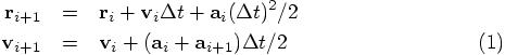
This is still the same leapfrog scheme, although represented in a different
way. Notice that the increment in  is given by the time step multiplied by
 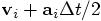 , effectively equal to
  . Similarly, the increment in
 is given by the time step
multiplied by
is given by the time step
multiplied by 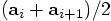 ,
effectively equal to the intermediate value
,
effectively equal to the intermediate value  . In conclusion, although both positions and
velocities are defined at integer times, their increments are governed by
quantities approximately defined at half-integer values of time.
. In conclusion, although both positions and
velocities are defined at integer times, their increments are governed by
quantities approximately defined at half-integer values of time.
Time reversibility
Alice: A great summary! I can see that you have taught numerical integration classes before. At this point an attentive student might be surprised by the difference between the two descriptions, which you claim to describe the same algorithm. They may doubt that they really address the same scheme.
Bob: How would you convince them?
Alice: An interesting way to see the equivalence of the two descriptions is to note the fact that the first two equations are explicitly time-reversible, while it is not at all obvious whether the last two equations are time-reversible. For the two systems to be equivalent, they’d better share this property. Let us inspect.
Starting with the first set of equations, even though it may be obvious,
let us write out the time reversibility. We will take one step forward,
taking a time step  , to
evolve
, to
evolve  to
to 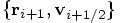 , and then we will take one
step backward, using the same scheme, taking a time step
, and then we will take one
step backward, using the same scheme, taking a time step  . Clearly, the time will return
to the same value since
. Clearly, the time will return
to the same value since 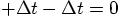 ,
but we have to inspect where the final positions and velocities
,
but we have to inspect where the final positions and velocities  are indeed equal to their
initial values
are indeed equal to their
initial values  . Here is
the calculation, resulting from applying the first set of equation twice:
. Here is
the calculation, resulting from applying the first set of equation twice:
In an almost trivial way, we can see clearly that time reversal causes both positions and velocities to return to their old values, not only in an approximate way, but exactly. In a computer application, this means that we can evolve forward a thousand time steps and then evolve backward for the same length of time. Although we will make integration errors (remember, leapfrog is only second-order, and thus not very precise), those errors will exactly cancel each other, apart from possible round-off effects, due to limited machine accuracy.
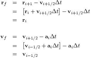
Now the real fun comes in, when we inspect the equal-time version, the second set of equations you presented:
In this case, too, we have exact time reversibility. Even though not immediately obvious from an inspection of your second set of equations, as soon as we write out the effects of stepping forward and backward, the cancellations become manifest.
Bob: A good exercise to give them. I’ll add that to my notes.
A New Driver
Alice: Now show me your leapfrog, I’m curious.
Bob: I wrote two new drivers, each with its own extended Body class. Let me show you the simplest one first. Here is the leapfrog driver integrator_driver1.rb:
 require "lbody.rb"

 include Math
 dt = 0.001            # time step
 dt_dia = 10           # diagnostics printing interval
 dt_out = 10           # output interval
 dt_end = 10           # duration of the integration
 #method = "forward"    # integration method
 method = "leapfrog"   # integration method

 STDERR.print "dt = ", dt, "\n",
       "dt_dia = ", dt_dia, "\n",
       "dt_out = ", dt_out, "\n",
       "dt_end = ", dt_end, "\n",
       "method = ", method, "\n"
 b = Body.new
 b.simple_read
 b.evolve(method, dt, dt_dia, dt_out, dt_end)
Same as before, except that now you can choose your integrator. The method evolve, at the end, now has an extra parameter, namely the integrator.
Alice: And you can supply that parameter as a string, either "forward" for our old forward Euler method, or "leapfrog" for your new leapfrog integrator. That is very nice, that you can treat that choice on the same level as the other choices you have to make when integrating, such as time step size, and so on.
Bob: And it makes it really easy to change integration method: one moment you calculate with one method, the next moment with another. You don’t even have to type in the name of the method: I have written it so that you can switch from leapfrog back to forward Euler with two key strokes: you uncomment the line
#method = "forward" # integration method
and comment out the line
method = "leapfrog" # integration method
Alice: It is easy to switch lines in the driver, but I’m really curious to see how you let Ruby actually make that switch in executing the code differently, replacing one integrator by another!
An Extended Body Class
Bob: Here is the new version of our Body class, in a file called lbody.rb with l for leapfrog. It is not much longer than the previous file body.rb, so let me show it again in full:
 require "vector.rb"

 class Body
   attr_accessor :mass, :pos, :vel

   def initialize(mass = 0, pos = Vector[0,0,0], vel = Vector[0,0,0])
     @mass, @pos, @vel = mass, pos, vel
   end
   def evolve(integration_method, dt, dt_dia, dt_out, dt_end)
     time = 0
     nsteps = 0
     e_init
     write_diagnostics(nsteps, time)

     t_dia = dt_dia - 0.5*dt
     t_out = dt_out - 0.5*dt
     t_end = dt_end - 0.5*dt
     while time < t_end
       send(integration_method,dt)
       time += dt
       nsteps += 1
       if time >= t_dia
         write_diagnostics(nsteps, time)
         t_dia += dt_dia
       end
       if time >= t_out
         simple_print
         t_out += dt_out
       end
     end
   end

   def acc
     r2 = @pos*@pos
     r3 = r2*sqrt(r2)
     @pos*(-@mass/r3)
   end
   def forward(dt)
     old_acc = acc
     @pos += @vel*dt
     @vel += old_acc*dt
   end

   def leapfrog(dt)
     @vel += acc*0.5*dt
     @pos += @vel*dt
     @vel += acc*0.5*dt
   end
   def ekin                        # kinetic energy
     0.5*(@vel*@vel)               # per unit of reduced mass
   end

   def epot                        # potential energy
     -@mass/sqrt(@pos*@pos)        # per unit of reduced mass
   end
   def e_init                      # initial total energy
     @e0 = ekin + epot             # per unit of reduced mass
   end

   def write_diagnostics(nsteps, time)
     etot = ekin + epot
     STDERR.print <<END
 at time t = #{sprintf("%g", time)}, after #{nsteps} steps :
   E_kin = #{sprintf("%.3g", ekin)} ,\
  E_pot =  #{sprintf("%.3g", epot)} ,\
  E_tot = #{sprintf("%.3g", etot)}
              E_tot - E_init = #{sprintf("%.3g", etot-@e0)}
   (E_tot - E_init) / E_init =#{sprintf("%.3g", (etot - @e0) / @e0 )}
 END
   end
   def to_s
     "  mass = " + @mass.to_s + "\n" +
     "   pos = " + @pos.join(", ") + "\n" +
     "   vel = " + @vel.join(", ") + "\n"
   end

   def pp               # pretty print
     print to_s
   end
   def simple_print
     printf("%24.16e\n", @mass)
     @pos.each{|x| printf("%24.16e", x)}; print "\n"
     @vel.each{|x| printf("%24.16e", x)}; print "\n"
   end

   def simple_read
     @mass = gets.to_f
     @pos = gets.split.map{|x| x.to_f}.to_v
     @vel = gets.split.map{|x| x.to_f}.to_v
   end
end
Minimal Changes
Alice: Before you explain to me the details, remember that I challenged you to write a new code while changing or adding at most a dozen lines? How did you fare?
Bob: I forgot all about that. It seemed so unrealistic at the time. But let us check. I first corrected this mistake about the mass factor that I had left out in the file body.rb. Then I wrote this new file lbody.rb. Let’s do a diff:
    |gravity> diff body.rb lbody.rb
    11c11
    <   def evolve(dt, dt_dia, dt_out, dt_end)
    - -
    >   def evolve(integration_method, dt, dt_dia, dt_out, dt_end)
    22c22
    <       evolve_step(dt)
    - -
    >       send(integration_method,dt)
    36c36
    <   def evolve_step(dt)
    - -
    >   def acc
    39c39,49
    <     acc = @pos*(-@mass/r3)
    - -
    >     @pos*(-@mass/r3)
    >   end
    >
    >   def forward(dt)
    >     old_acc = acc
    >     @pos += @vel*dt
    >     @vel += old_acc*dt
    >   end
    >
    >   def leapfrog(dt)
    >     @vel += acc*0.5*dt
    41c51
    <     @vel += acc*dt
    - -
    >     @vel += acc*0.5*dt
To wit: four lines from the old code have been left out, and twelve new lines appeared.
Alice: Only twelve! You did it, Bob, exactly one dozen, indeed.
Bob: I had not realized that the changes were so minimal. While I was playing around, I first added a whole lot more, but when I started to clean up the code, after it worked, I realized that most of my changes could be expressed in a more compact way.
Alice: Clearly Ruby is very compact.
Bob: Let me step through the code.