11. The Hermite Algorithm
Alice: I'm quite impressed with the large collection of integrators
we have built up. But perhaps it is time to move on, and adapt all of
them to the real N-body problem, now that we have their two-body form?
Bob: Yes, but there is one more integrator that I wanted to add to our
pile. I had mentioned the Hermite algorithm, when we started to look at
multiple-step methods, as an alternative to get fourth-order accuracy,
without using multiple steps and without using half steps. Actually,
coding it up was even simpler than I had expected. You could argue that
it is the simplest self-starting Fourth-Order Scheme, once you allow the
direct calculation of the jerk, in addition to that of the acceleration.
Alice: Can you show me first the idea behind the algorithm?
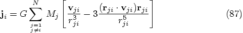
Bob: The trick is to differentiate Newton's gravitational equations of
motion
Note that the jerk has one very convenient property. Although the
expression above looks quite a bit more complicated than Newton's
original equations, they can still be evaluated through one pass over
the whole
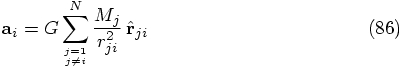
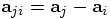
Alice: I see. So it is quite natural to differentiate Newton's
equations of motion just once, and then to use both the acceleration
and the jerk, obtained directly from Eqs. (86) and
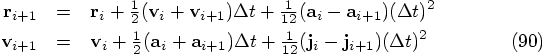
(87). Can you show me what the expressions for the
position and velocity look like, in terms of those two quantities?
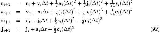
Bob: Here they are:
Bob: Yes, I think you can look at the Hermite scheme as a generalization
of the leapfrog, in some sense. If you neglect the
terms that are quadratic in
Alice: Yes, since in that case you can write the terms linear in
In general, you might have expected
two extra terms, one of order
The question is, can we understand why the remaining terms are what
they are, and especially why they can be written in such a simple way?
Bob: I thought you would ask that, and yes, this time I've done my
homework, anticipating your questions. Here is the simplest derivation
that I could come up with.
Since we are aiming at a fourth-order scheme, all we have to do is to
expand the position and velocity up to fourth-order terms in the time
step
Alice: You mean that a term proportional to, say,
Bob: Exactly. Here it is, in equation form:
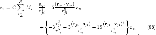
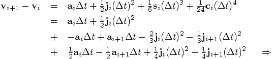
Bob: We can now eliminate snap and crackle at time
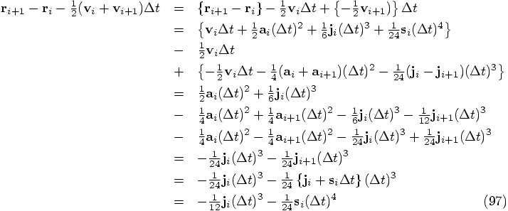
The only thing left to do is to check the expression for the position,
the first line in Eq. (90). Let us bring everything to
the left-hand side there, except the acceleration terms. In other words,
let us split off the leapfrog expression, and see what is left over:
Alice: Great! Can you show me how you have implemented this scheme?
Bob: It was surprisingly simple. I opened a file called hbody.rb,
with yoshida6.rb as my starting point. And all I had to do was
to add a method jerk to compute the jerk, and then a method hermite
to do the actual Hermite integration.
The jerk method, in fact, is rather similar to the acc method:
apart from the last line:
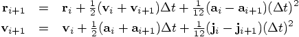
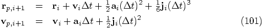
Alice: Before you show me the integrator, let me look at the equations
again, which you have derived, to get an idea as to what to expect. Here
they are:
In other words, these are implicit equations for the position and the
velocity. How do you deal with them?
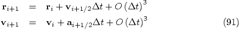
Bob: Through iteration. I first determine trial values for the position
and velocity, simply by expanding both as a Taylor series, using only what
we know at time
However, I am worried about that velocity term in the first line on
the right-hand side of Eq. (102). According to
Eq. (101), your predicted velocity has an error of order
Bob: Huh, you're right. How can that be? Is that really what I
implemented? That cannot be correct. I'd better check my code.
Here it is, the hermite method that is supposed to do the job:
Ah, I see what I did! Of course, and now I remember also why I did it that
way. I was wrong in what I wrote above. I should have written
Eq. (102) as follows:
11.1. A Self-Starting Fourth-Order Scheme
 .
.
 -body system. This is no longer true for
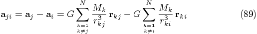
higher derivatives. For example, we can obtain the fourth derivative
of the position of particle
-body system. This is no longer true for
higher derivatives. For example, we can obtain the fourth derivative
of the position of particle  , the snap, by
differentiating the above equation one more time:
, the snap, by
differentiating the above equation one more time:
 , and this is the
expression that thickens the plot. Unlike the
, and this is the
expression that thickens the plot. Unlike the  and
and  expressions, that are given by the initial
conditions,
expressions, that are given by the initial
conditions,  has to be calculated from the
positions and velocities. However, this calculation does not only
involve the pairwise attraction of particle
has to be calculated from the
positions and velocities. However, this calculation does not only
involve the pairwise attraction of particle  on particle
 , but in fact all pairwise attractions of all particles
on each other! This follows immediately when we write out what the
shorthand implies:
, but in fact all pairwise attractions of all particles
on each other! This follows immediately when we write out what the
shorthand implies:
 -body system,
summing over both indices
-body system,
summing over both indices  and
and  in order
to compute a single fourth derivative for the position of particle
in order
to compute a single fourth derivative for the position of particle
 .
.
11.2. A Higher-Order Leapfrog Look-Alike
 , you get exactly
the leapfrog back.
, you get exactly
the leapfrog back.
 as effectively half-step quantities, up to
higher powers in
as effectively half-step quantities, up to
higher powers in  :
:
 and one of order
 , for the position, as well as for the velocity.
Instead there is just one term, in each case. And that one term is
written with a misleading factor of
, for the position, as well as for the velocity.
Instead there is just one term, in each case. And that one term is
written with a misleading factor of  , but of
course there is at least one more factor
, but of
course there is at least one more factor  lurking
in the factor
lurking
in the factor  , which to first order
in
, which to first order
in  is nothing else than
  ;
or
;
or  for that matter. And similarly, there
is a factor
for that matter. And similarly, there
is a factor  hidden in
  .
.
 , while we can drop one factor of
 for the acceleration, and two factors for the jerk,
to the same order of consistency.
for the acceleration, and two factors for the jerk,
to the same order of consistency.
 in the jerk would be derived from a term proportional to
 in the velocity or from a term proportional to
 in the position, both of which are beyond our
approximation.
in the position, both of which are beyond our
approximation.
11.3. A Derivation
 ,
expressing them in terms of the acceleration and jerk at times
,
expressing them in terms of the acceleration and jerk at times
 and
and  , using the last two lines of
Eq. (92). This gives us for the snap
, using the last two lines of
Eq. (92). This gives us for the snap


 in the last
term.
in the last
term.


11.4. Implementation
   def acc
     r2 = @pos*@pos
     r3 = r2*sqrt(r2)
     @pos*(-@mass/r3)
   end
   def jerk
     r2 = @pos*@pos
     r3 = r2*sqrt(r2)
     (@vel+@pos*(-3*(@pos*@vel)/r2))*(-@mass/r3)
   end
 . However, on the right-hand side you rely also on
the acceleration and jerk at time
. However, on the right-hand side you rely also on
the acceleration and jerk at time  , which you can
only compute after you have determined the position and velocity at
time
, which you can
only compute after you have determined the position and velocity at
time  . In addition, you also have the future
velocity at the right-hand side as well.
. In addition, you also have the future
velocity at the right-hand side as well.
 , which are the position, velocity,
acceleration and jerk. In fact, this is a type of predictor-corrector
method. If I express those trial values with a subscript p, I start
with:
, which are the position, velocity,
acceleration and jerk. In fact, this is a type of predictor-corrector
method. If I express those trial values with a subscript p, I start
with:
 , I can solve the
equations for the corrector step, where I indicate the final values
for the position and velocity at time
, I can solve the
equations for the corrector step, where I indicate the final values
for the position and velocity at time  with a
subscript s :
with a
subscript s :

 in the velocity, and terms
of order
in the velocity, and terms
of order  in the position, but those predictor values
for position and velocity are only used to compute acceleration and jerk,
terms that are always multiplied with factors of
in the position, but those predictor values
for position and velocity are only used to compute acceleration and jerk,
terms that are always multiplied with factors of  ,
so the resulting errors are of order
,
so the resulting errors are of order  . Good!
 , so by multiplying that with a single factor
 , you wind up with an error of order
 , which is certainly not acceptable.

 and
and  in the normal order,
and I got a pretty bad energy behavior, until I realized that I should switch
the order of computations. How easy to make a quick mistake and a
quick fix, and then to forget all about it!
in the normal order,
and I got a pretty bad energy behavior, until I realized that I should switch
the order of computations. How easy to make a quick mistake and a
quick fix, and then to forget all about it!
 . High time to go to large
  values.