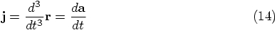
4. A Fourth-Order Integrator
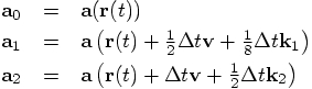
Bob: Now it is really time to show off my fourth-order integrator.
Alice: Can you show me again the code?
Bob: Here it is:
Alice: That's quite a bit more complicated. I see coefficients of
1/6 and 1/3 and 2/3. How did you determine those?
Bob: I just looked them up in a book. There are several ways to
choose those coefficients. Runge-Kutta formulas form a whole family,
and the higher the order, the more choices there are for the
coefficients. In addition, there are some extra simplifications that
can be made in the case of a second order differential equation where
there is no dependence on the first derivative.
Alice: As in the case of Newton's equation of motion, where the
acceleration is dependent on the position, but not on the velocity.
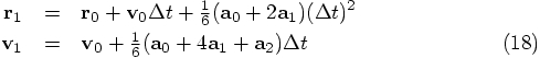
Bob: Exactly. Here are the equations. They can be found in that
famous compendium of equations, tables and graphs: Handbook of
Mathematical Functions, by M. Abramowitz and I. A. Stegun,
eds. [Dover, 1965]. You can even find the pages on the web now.
Here is what I copied from a web page:
Alice: Quite a bit more complex than the second order one.
Bob: Yes, and of course it is written in a rather different form
than the way I chose to implement it. I preferred to stay close to the
same style in which I had written the leapfrog and second-order Runge
Kutta. This means that I first had to rewrite the Abramowitz and
Stegun expression.
Alice: Let's write it out specifically, just to check what you did.
I know from experience how easy it is to make a mistake in these kinds
of transformations.
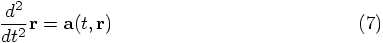
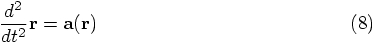
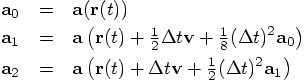
Bob: So do I! Okay, the book starts with the differential equation:
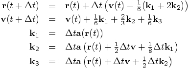
Alice: Let us rewrite their set of equations in terms of the
dictionary you just provided. And instead of dt it is better to
write
We can now rewrite the first two of Abramowitz and Stegun's equations as:
Bob: Yes, that was how I derived my code, but I must admit, I did
not write it down as neatly and convincingly as you just did.
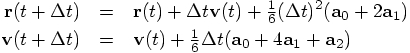
Alice: So yes, you have indeed implemented Abramowitz and Stegun's
fourth-order Runge-Kutta scheme. But wait a minute, what
you found here, equation 22.5.22, shows a right-hand side with a
stated position error of order
Bob: Hey, that is right. If you make
Alice: Could it be a misprint?
Bob: Anything is possible, though here that is not very likely. This
is such a famous book, that you would expect the many readers to have
debugged the book thoroughly.
Alice: Let's decide for ourselves what is true and what is not.
Bob: Yes. And either way, whatever the outcome, it will be a good
exercise for the students. Let's first test it numerically.
Alice: Fine with me. But then I want to derive it analytically as well,
to see whether we really can understand the behavior of the numerical
results from first principles.
And hey, I just noticed that the expression for the velocity in
equation 22.5.22 does not have any error estimate. For the scheme
to be really fourth-order, not only should the error per step in the
first line be of order
Bob: Whether those facts are true or not, that will be easy to figure
out numerically. Let us start again with a time step of 0.001, for a
duration of ten time units.
Alice: Just to compare, why don't you run them for all four schemes.
Bob: I am happy to do so. And while we are not sure yet whether our
higher-order Runge-Kutta scheme is 3rd order or 4th order, let me
continue to call it 4th order, since I've called it rk4 in my
code. If it turns out that it is 3rd order, I'll go back and rename
it to be rk3.
Alice: Fair enough.
Bob: Okay: forward Euler, leapfrog, 2nd order R-K, and hopefully-4th
order R-K:
Bob: The leapfrog does better:
Bob: Time for second-order Runge-Kutta:
Bob: Here is the answer:
Bob: Yes, I'm really glad I threw that integrator into the menu.
The second-order Runge-Kutta doesn't fare as well as the leapfrog, at
least for this problem, even though they are both second-order. But
the hopefully-fourth-order Runge-Kutta wins hands down.
Alice: Let's make the time step ten times smaller:
Alice: Well done. And, by the way, this does suggest that the scheme
that you copied from that book is indeed fourth-order. It almost seems
better than fourth order.
Bob: Let me try a far larger time step, but a much shorter duration,
so that we don't have to integrate over a complicated orbit. How
about these two choices. First:
Bob: This proves it. And I can keep the name rk4,
since it lives up to its claim. Good!
Alice: At least it comes close to living up to its name, and it
sort-of proves it.
Bob: What do you mean with `comes close'? What more proof would you
like to have?
Alice: I would still be happier if I could really prove it,
with pen and paper, rather than through the plausibility of numerical
experimentation.
Bob: Go ahead, if you like!
Alice: Let us take your implementation
and let us determine analytically what the first five terms in a Taylor
series in dt look like. We can then see directly whether the error term
is proportional to
To start with, let us look at your variable a2, which is the
acceleration after a time step dt, starting from an initial
acceleration a0. A Taylor expansion can approximate
a2 as:
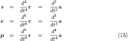
Bob: The first derivative of the acceleration,
Bob: It may be more difficult to come up with terms for the unevenness
in the jerk.
Alice: Actually, I saw somewhere that someone had used the words
snap, crackle, and pop, to describe the next three terms.
Bob: As in the rice crispies? Now that will confuse astronomers
who did not grow up in the United States! If they haven't seen the
rice crispy commercials, they will have no clue why we would use those
names. And come to think of it, I don't have much of a clue yet either.
Figure 1: Snap, Crackle, and Pop
Bob: Okay, now I get the drift of the argument. A sudden snap comes to
mind, as a change in jerk. And what changes its state more suddenly than
a snap? Well, perhaps something that crackles, although that is pushing
it a bit. But a pop is certainly a good word for something that
changes high derivatives of positions in a substantial way!
Alice: Okay, let's make it official:
Alice: And your other variable a1, which indicates the acceleration
after only half a time step, now becomes:
Alice: Yes. These two lines translate to:
Alice: Or so it seems. But I must admit, I'm not completely comfortable.
Bob: Boy, you're not easy to please! I was ready to declare victory
when we had our numerical proof, and you convinced me to do the additional
work of doing an analytical check. If it were up to me, I would believe
numerics over analytics, any day. Seeing is believing, the proof is
in the pudding, and all that.
Alice: Well, it really is better to have both a numerical
demonstration and an analytical proof. It is just too easy to be
fooled by coincidences or special cases, in numerical demonstrations.
And at the same time it is also easy to make a mistake in doing
analytical checks. So I think it is only wise to do both, especially
with something so fundamental as an N-body integrator.
And I'm glad we did. But something doesn't feel quite right. Let me
just review what we have done. We first expanded the orbit in a Taylor
series, writing everything as a function of time. Then we showed that
the orbit obeyed the equations of motion, and . . . .
Bob: . . . and then you looked shocked.
Alice: Not only do I look shocked, I am shocked! How could we make
such a stupid mistake!?!
Bob: I beg your pardon?
Alice: There is something quite wrong with the Taylor series I wrote
down in Eq. (13).
Bob: I looks like a perfectly fine Taylor series to me. All the
coefficients are correct, and each next term is a higher derivative
of the acceleration. What could possibly be wrong with it?
Alice: Formally it looks right, yes, that is exactly what is so misleading
about it. But it is dead wrong.
Bob: Give me a hint.
Alice: Here is the hint. This Taylor series is formally correct, alright,
for the case where you really know the function on the left hand side, and
you really know all the derivatives on the right hand side. In that case,
what you leave out is really fifth-order in
Bob: So?
Alice: The problem is, we don't have such idealized information.
Look at Eq. (16), or no, even better, look at Eq. (17).
Bob: I must be missing something. Here is Eq. (17) again:
Alice: Yes, formally, true. But where do we apply it to? That's
the problem. Let us recall how we actually compute
Now tell me, how accurate is this expression for
Bob: It is based on the position calculated in the third line of the body
of the code, which is second order accurate in dt. So this means
that a1 must be second-order accurate at this point. But that's
okay, since a2 is already higher-order accurate, since it
uses the information of a1 which was used to construct a better
approximation for the position, in the fifth line of the code. And then
the next line presumably gives an even better approximation. My guess
would be that, while a1 is second-order accurate in dt,
a2 is third-order accurate, and the next acceleration evaluation,
at the beginning of the next step, will then be fourth-order accurate;
that will be a0 in the following round. This is the whole point
of a Runge-Kutta approach: you bootstrap your way up to the required
accuracy.
Alice: Yes, I agree with all that, but that is far more than we need right
now. Let's just stick with a1, and only a1. It was
second-order accurate in dt, you just said. Now how in the world
can a second-order accurate formula give any information in a comparison
with four subsequent derivatives in Eq. (17) ???
Bob: Aaaaah, now I see what you are driving at. Well, I suppose it can't.
Alice: And similarly, your guess was that a2 was only third-order
accurate, right? So it does not make sense to require it to fit
snugly up to fourth-order in Eq. (16), which is the expression
we started with, Eq. (13).
Bob: Well, if you put it that way, I must admit, no, that would not make
sense. How tricky!
Alice: How tricky indeed! I was fully convinced that we were doing the
right thing.
Bob: So was I. How dangerous, to rely on formal expressions!
Alice: And now that we have spotted the fallacy in our reasoning, we can
see what we should have done: in Eq. (13), we should have
expanded not only the right-hand side, but also the left-hand side, given
that there are approximations involved there as well. Only after
doing that, can we equate both sides in all honesty!
Bob: Yes, that is the only way, that much is clear now. Okay, you've
convinced me. We really should keep track of all the approximations involved.
Alice: Now let's do it! 4.1. Coefficients
4.2. Really Fourth Order?

 , and their
f becomes our acceleration vector
, and their
f becomes our acceleration vector  . Also, their
 becomes our velocity vector
  . Finally, their h is
our time step dt.
. Finally, their h is
our time step dt.
 , since dt is not an infinitesimal quantity
here, but a finite time interval. This then gives us:
, since dt is not an infinitesimal quantity
here, but a finite time interval. This then gives us:
 ,
,  , and
, and  as follows, taking the right hand sides of the last three equations above,
but without the
as follows, taking the right hand sides of the last three equations above,
but without the  factor:
 ,
,
 , and
, and  , we can eliminate all
 values from the right hand side:
 -- which would suggest
that the scheme is only third-order accurate.
-- which would suggest
that the scheme is only third-order accurate.
 smaller,
the number of steps will go up according to
smaller,
the number of steps will go up according to  , and
therefore the total error for a given problem will grow proportionally
to
, and
therefore the total error for a given problem will grow proportionally
to 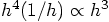 . This would indeed imply that
this method is third-order. But that would be very unusual. In all
text books I've seen, you mostly come across second-order and
fourth-order Runge-Kuttas. While you certainly can construct a
third-order version, I wouldn't have expected Abramowitz and Stegun to
feature one. Besides, look at the last expression for the velocity.
Doesn't that resemble Simpson's rule, suggesting fourth-order accuracy.
I'm really puzzled now.
. This would indeed imply that
this method is third-order. But that would be very unusual. In all
text books I've seen, you mostly come across second-order and
fourth-order Runge-Kuttas. While you certainly can construct a
third-order version, I wouldn't have expected Abramowitz and Stegun to
feature one. Besides, look at the last expression for the velocity.
Doesn't that resemble Simpson's rule, suggesting fourth-order accuracy.
I'm really puzzled now.
 , but the second line should
also have an error of order
, but the second line should
also have an error of order  . I want to see whether
we can derive both facts, if true.
. I want to see whether
we can derive both facts, if true.
4.3. Comparing the Four Integrators
 |gravity> ruby integrator_driver2d.rb < euler.in
 dt = 0.001
 dt_dia = 10
 dt_out = 10
 dt_end = 10
 method = forward
 at time t = 0, after 0 steps :
   E_kin = 0.125 , E_pot =  -1 , E_tot = -0.875
              E_tot - E_init = 0
   (E_tot - E_init) / E_init =-0
 at time t = 10, after 10000 steps :
   E_kin = 0.0451 , E_pot =  -0.495 , E_tot = -0.45
              E_tot - E_init = 0.425
   (E_tot - E_init) / E_init =-0.486
   1.0000000000000000e+00
   2.0143551288236803e+00  1.6256533638564666e-01
  -1.5287552868811088e-01  2.5869644289548283e-01
Alice: Ah, this is the result from the forward Euler algorithm,
because the fifth line of the output announces that this was the
integration method used. As we have seen before, energy conservation
has larger errors. We have an absolute total energy error of 0.425,
and a relative change in total energy of -0.486. I see that you
indeed used dt = 0.001 from what is echoed on the first line
in the output. And yes, for these choices of initial conditions and
time step size we had seen that things went pretty badly.
 |gravity> ruby integrator_driver2e.rb < euler.in
 dt = 0.001
 dt_dia = 10
 dt_out = 10
 dt_end = 10
 method = leapfrog
 at time t = 0, after 0 steps :
   E_kin = 0.125 , E_pot =  -1 , E_tot = -0.875
              E_tot - E_init = 0
   (E_tot - E_init) / E_init =-0
 at time t = 10, after 10000 steps :
   E_kin = 0.554 , E_pot =  -1.43 , E_tot = -0.875
              E_tot - E_init = 3.2e-07
   (E_tot - E_init) / E_init =-3.65e-07
   1.0000000000000000e+00
   5.9946121055215340e-01 -3.6090779482156415e-01
   1.0308896785838775e+00  2.1343145669114691e-01
Alice: Much better indeed, as we had seen before. A relative energy
error of  is great, an error much less
than one in a million.
is great, an error much less
than one in a million.
 |gravity> ruby integrator_driver2f.rb < euler.in
 dt = 0.001
 dt_dia = 10
 dt_out = 10
 dt_end = 10
 method = rk2
 at time t = 0, after 0 steps :
   E_kin = 0.125 , E_pot =  -1 , E_tot = -0.875
              E_tot - E_init = 0
   (E_tot - E_init) / E_init =-0
 at time t = 10, after 10000 steps :
   E_kin = 0.555 , E_pot =  -1.43 , E_tot = -0.875
              E_tot - E_init = 6.02e-05
   (E_tot - E_init) / E_init =-6.88e-05
   1.0000000000000000e+00
   5.9856491479183715e-01 -3.6183772788952318e-01
   1.0319067591346045e+00  2.1153690796461602e-01
Alice: Not as good as the leapfrog, but good enough. What I'm curious
about is how your hopefully-fourth-order Runge-Kutta will behave.
 |gravity> ruby integrator_driver2g.rb < euler.in
 dt = 0.001
 dt_dia = 10
 dt_out = 10
 dt_end = 10
 method = rk4
 at time t = 0, after 0 steps :
   E_kin = 0.125 , E_pot =  -1 , E_tot = -0.875
              E_tot - E_init = 0
   (E_tot - E_init) / E_init =-0
 at time t = 10, after 10000 steps :
   E_kin = 0.554 , E_pot =  -1.43 , E_tot = -0.875
              E_tot - E_init = -2.46e-09
   (E_tot - E_init) / E_init =2.81e-09
   1.0000000000000000e+00
   5.9961758437074986e-01 -3.6063455639926667e-01
   1.0308068733946525e+00  2.1389536225475009e-01
Alice: What a difference! Not only do we have much better energy
conservation, on the order of a few times  ,
also the positional accuracy is already on the level of a few times
,
also the positional accuracy is already on the level of a few times
 , when we compare the output with our most
accurate previous runs. And all that with hardly any waiting time.
, when we compare the output with our most
accurate previous runs. And all that with hardly any waiting time.
4.4. Fourth Order Runge-Kutta
 |gravity> ruby integrator_driver2h.rb < euler.in
 dt = 0.0001
 dt_dia = 10
 dt_out = 10
 dt_end = 10
 method = rk4
 at time t = 0, after 0 steps :
   E_kin = 0.125 , E_pot =  -1 , E_tot = -0.875
              E_tot - E_init = 0
   (E_tot - E_init) / E_init =-0
 at time t = 10, after 100000 steps :
   E_kin = 0.554 , E_pot =  -1.43 , E_tot = -0.875
              E_tot - E_init = -8.33e-14
   (E_tot - E_init) / E_init =9.52e-14
   1.0000000000000000e+00
   5.9961755488723312e-01 -3.6063458344261029e-01
   1.0308069102701605e+00  2.1389530419780176e-01
Bob: What a charm! Essentially machine accuracy. This makes it
pretty obvious that fourth-order integrators win out hands down, in
problems like this, over second-order integrators. Higher order
integrators may be even faster, but that is something we can explore
later.
 |gravity> ruby integrator_driver2i.rb < euler.in
 dt = 0.1
 dt_dia = 0.1
 dt_out = 0.1
 dt_end = 0.1
 method = rk4
 at time t = 0, after 0 steps :
   E_kin = 0.125 , E_pot =  -1 , E_tot = -0.875
              E_tot - E_init = 0
   (E_tot - E_init) / E_init =-0
 at time t = 0.1, after 1 steps :
   E_kin = 0.129 , E_pot =  -1 , E_tot = -0.875
              E_tot - E_init = 1.75e-08
   (E_tot - E_init) / E_init =-2.01e-08
   1.0000000000000000e+00
   9.9499478923153439e-01  4.9916431937376750e-02
  -1.0020915515250550e-01  4.9748795077019681e-01
And then:
 |gravity> ruby integrator_driver2j.rb < euler.in
 dt = 0.01
 dt_dia = 0.1
 dt_out = 0.1
 dt_end = 0.1
 method = rk4
 at time t = 0, after 0 steps :
   E_kin = 0.125 , E_pot =  -1 , E_tot = -0.875
              E_tot - E_init = 0
   (E_tot - E_init) / E_init =-0
 at time t = 0.1, after 10 steps :
   E_kin = 0.129 , E_pot =  -1 , E_tot = -0.875
              E_tot - E_init = 1.79e-12
   (E_tot - E_init) / E_init =-2.04e-12
   1.0000000000000000e+00
   9.9499478009063858e-01  4.9916426216739009e-02
  -1.0020902861389222e-01  4.9748796005932194e-01
Alice: The time step went down by a factor of 10, and the energy
conservation got better by a factor of almost exactly  .
We really seem to have a fourth order integration scheme.
.
We really seem to have a fourth order integration scheme.
4.5. Snap, Crackle, and Pop
 , as the book claims, or
  ,
as our calculations indicate.
,
as our calculations indicate.

 , namely at the beginning of our time step.
 ,
is sometimes called the jerk. How about the following notation:
,
is sometimes called the jerk. How about the following notation:

4.6. An Attempt at an Analytical Proof


     @pos = old_pos + vel*dt + (a0+a1*2)*(1/6.0)*dt*dt
     @vel = vel + (a0+a1*4+a2)*(1/6.0)*dt


 are
perfectly correct, and the error starts in the
are
perfectly correct, and the error starts in the  term,
where the Taylor series coefficient would have been
term,
where the Taylor series coefficient would have been  .
So the leading error terms are:
.
So the leading error terms are:
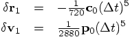
4.7. Shocked
 .
.

 .
Here is your implementation of rk4 again:
.
Here is your implementation of rk4 again:
 ,
or in the terms of the code, for a1
,
or in the terms of the code, for a1