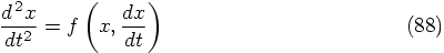
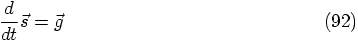
3. Second-Order Differential Equations
Alice: Now that we know how to solve a first-order differential equation, we
can extend our methods immediately to treat the case of a general
second-order differential equation
Bob: Wouldn't it be simpler to restrict ourselves immediately to
the type of equations we are dealing with in stellar dynamics, without
any velocity dependence in the forces?
Alice: I would prefer to hold off just a bit, because the simplest way
to treat second-order equations is by following the same recipe as we did
before. In that case, velocity dependence does not pose any problems.
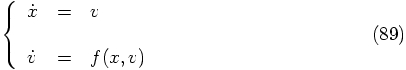
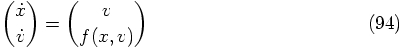
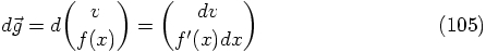
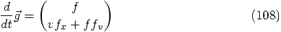
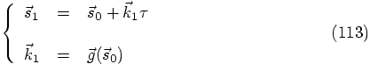
The second-order equation above can be rewritten as a system of two
first-order differential equations:
Bob: Ah, that is a nice short-cut. Let's do that, and then we should
be able to use all the results from the previous chapters immediately!
Alice: We'll think have to put in some thought, since not all scalar
equations generalize in an obvious way to the vectorial case, but I agree
that it would probably be a good guide line.
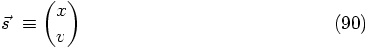
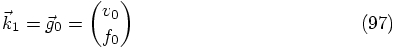
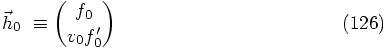
Okay, to introduce vector notation, let us define:
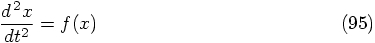
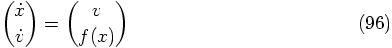
Bob: Fine, but let's not linger too long! And please, let us drop the
velocity dependence in the forces. Life is complicated enough as it is.
Alice: Okay, okay, we'll work with
In order to compute
Bob: presumably that is simply
Alice: Not so fast! You have not specified what you mean with
that notation. The left-hand side is a vector, while the right-hand
side suggests the product of two vectors. What does it mean?
Bob: Hmm. I hadn't thought about that. Good question.
Alice: If it would be an inner product, the left hand side should
be a scalar. If, however, it is a tensor product, the left hand side
should be a tensor. In neither case does it produce a vector.
Bob: Again, good point. Wel, in case of doubt, write it out!
What does it look like in components?
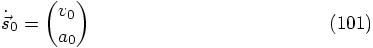
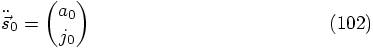
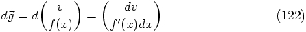
Alice: Let us check. The most intuitive approach would be to start
with a small variation in
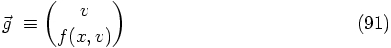
Alice: Yes. And even if you would have allowed me to retain a velocity
dependence in the force, we would still have wound up with a vector, but
in this case we would have:
Alice: If you insist. At least the notation above will point the way for
further generalizations, whenever we want to go that route.
Bob: Thanks!
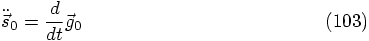
Alice: Let us introduce the symbol
Bob: Quite a bit of work to regain Forward Euler!
Alice: Yes, and we might have guessed the result, but when we move
on to using two force evaluations per step, things will undoubtedly
get messier.
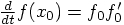
As before, after a first evaluation of the
right-hand side of the differential equation, we can perform a
preliminary integration in time, after which we can evaluate the
right-hand side again, at a new position:
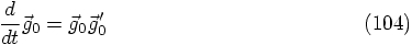
Alice: To sum up: developing
Bob: So, now we're done, and we can move on!
Alice: Yes, but let us put all our results on the table first.
To summarize, we can write:
Alice: My pleasure! Starting with
Bob: I find this a lot more understandable that the vector notation.
And for practical application, let's look at a couple special case.
For
Bob: How so?
Alice: The expression for
Bob: And so is the expression for
Alice: Ah, the word exact is important here! While it is true that
Bob: Tricky! So we are dealing with an almost-leapfrog scheme, where
the last force calculation is based on a predicted value for the new
position, instead of the corrected value.
Alice: Yes, that's a good way of putting it. And all this can serve
as an invitation to go beyond the straightforward generalizations of the
Runge-Kutta schemes for first-order differential equations. It is time
to look at more imaginative schemes, that treat position and velocity in
different ways! 3.1. Formulating the Problem
 exerted on a particle depends
explicitly on both the position and the velocity of that particle.
An example of such a force is the motion of a mass point under the
influence of friction. Indeed, our physical interpretation of the
case of a first-order differential equation followed from the above
form in the limit of infinitely strong friction, where the
velocity-dependent term dominated completely. Another example would
be the force that is felt by an electron moving in an electromagnetic
field (where
exerted on a particle depends
explicitly on both the position and the velocity of that particle.
An example of such a force is the motion of a mass point under the
influence of friction. Indeed, our physical interpretation of the
case of a first-order differential equation followed from the above
form in the limit of infinitely strong friction, where the
velocity-dependent term dominated completely. Another example would
be the force that is felt by an electron moving in an electromagnetic
field (where  would have be interpreted as a three-dimensional
vector, a point we will come back to later in this chapter).
would have be interpreted as a three-dimensional
vector, a point we will come back to later in this chapter).
3.2. Vector Notation

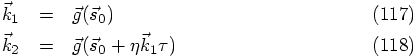
3.3. One Force Evaluation per Step
 then. Now,
everything we have done so far carries over directly to the
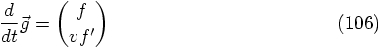
case of two coupled differential equations. To show this, let us
repeat the same derivation, but now in vector form. At the start of a
time step, we evaluate the right-hand side of the differential
equation at
then. Now,
everything we have done so far carries over directly to the
case of two coupled differential equations. To show this, let us
repeat the same derivation, but now in vector form. At the start of a
time step, we evaluate the right-hand side of the differential
equation at  :
:


 at time 0.
 .
.
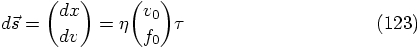
3.4. Not So Fast
 .
.
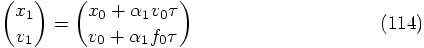
 , which can be
expressed as
, which can be
expressed as

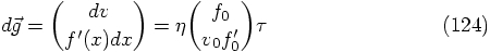
 and
and
 . This would give us
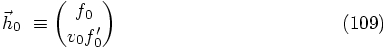
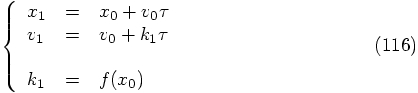
3.5. Forward Euler in Vector Form
 for the right-hand
side of Eq. (106), at time 0:
for the right-hand
side of Eq. (106), at time 0:

 matches trivially, and the first
condition arises from the term linear in
matches trivially, and the first
condition arises from the term linear in  :
:


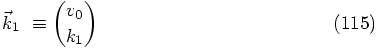
 for the vector and
the last componenent, again to avoid introducing yet more new letters.
With this notation, we can write Eq. (111) in a more
traditional form as:
for the vector and
the last componenent, again to avoid introducing yet more new letters.
With this notation, we can write Eq. (111) in a more
traditional form as:
 term in Eq. (110).
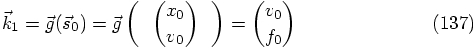
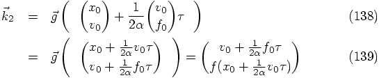
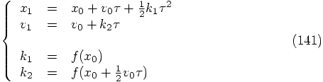
3.6. Two Force Evaluations per Step
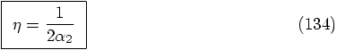
 . The coefficient
for each term is, as yet, arbitrary, so let us parametrize them as
follows:
. The coefficient
for each term is, as yet, arbitrary, so let us parametrize them as
follows:


 and
and  , can now be plugged back into the
definition of
, can now be plugged back into the
definition of 

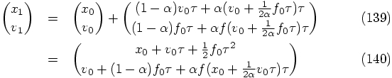
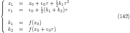
3.7. Putting Everything Together
 in a Taylor series around
  gives:


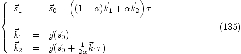
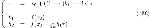
 as follows:

 in
Eqs. (128) and (130), we have to insist that
in
Eqs. (128) and (130), we have to insist that


 , we would like to satisfy:

 .
.
3.8. Summary
 :
:
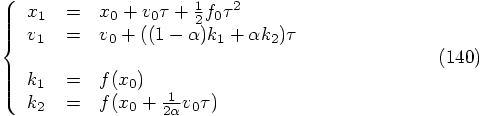
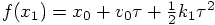
3.9. Two Examples
 we find
 we find
 is exactly the same as what
we have used when we implemented the leapfrog.
is exactly the same as what
we have used when we implemented the leapfrog.
 . The whole idea of
leapfrogging is to advance the velocity with an acceleration that is the
exact average of the force calculation at the beginning and at the end
of the step.
. The whole idea of
leapfrogging is to advance the velocity with an acceleration that is the
exact average of the force calculation at the beginning and at the end
of the step.
 is the force evaluation at the beginning of the step,
the exact force calculation at the end of the step would be
is the force evaluation at the beginning of the step,
the exact force calculation at the end of the step would be
 . However, in
our scheme above,
. However, in
our scheme above, 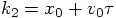 , and the last term
is missing.
, and the last term
is missing.