2. N-Body Integrators
Alice: Yes, I get the idea, and that all makes a lot of sense.
And now that we understand how the data get read in, let's see what will happen
with them.
In rknbody1.rb, I see that you have shifted all the integration
methods from the Body to the Nbody class, as well as the evolve function
that calls them.
Bob: The evolve function orchestrates the whole integration process, and
it is called by the driver, which only knows about the one Nbody
instance that it has created. So it is logical to put the evolve
method inside the Nbody class. And since evolve calls the various
integration methods, it also seemed logical to have leapfrog,
rk2, and so on, reside there.
Alice: I could imagine an alternative, where each particle is given the
freedom to use its own integration method, in which case you would
want to shift those methods back into the Body class, but that would make
more sense when you use an individual time step algorithm, where each
particle has its own time step length. For the simple shared time step case
that we are starting with, your choice is surely the best.
Bob: I could imagine many things, but coding them takes more time than
imagining them! I do like the idea of relatively autonomous particles,
integrating themselves as they want, with stars in denser regions having
perhaps more specialized integrators, but not today.
Alice: Looking at evolve, I see almost exactly the same function that
we used for the two-body problem. The only difference is that now the
time is an instance variable for the Nbody class, which means that we
don't have to pass the time as an argument to the write_diagnostics
method.
Bob: Yes. If I would have left the time as a normal variable that would
be passed around, the evolve method would have been exactly the same.
A nice example of recycling code: whether you are dealing with one
pseudo particle or with N particles, the top level instructions are
basically the same.
Alice: But of course the actual work is different, and in our case more
complicated. The forward Euler implementation is a bit hard to recognize,
at first sight. Let me start with the new leapfrog method, which
looks more familiar. The two-body version was:
while now we have
This is easy to understand: for each body, basically the same actions are
taken as was the case for our single pseudo-body, containing the relative
position information for the two-body case.
Bob: The difference being that, invisibly at this level, the Body
method acc, which computes the acceleration, has to ask all other
particles for their position.
Alice: Indeed, acc has grown quite a bit bigger. In the two-body case,
we started with
and your new N-body version reads:
Bob: The main difference is the loop that our body has to execute over
all other bodies. It is here that I am using my backpointer @nb
that links back to the parent Nbody instance. In that way, the array of
bodies becomes visible for our particular body as @nb.body, and
it is this array over which we iterate using the familiar each construct.
Alice: And you are excluding the body itself from the loop, to avoid
getting an infinitely large self interaction, through the line:
But what exactly are you comparing? I am used to the C notation where
== compares two numbers. In Ruby too, when both numbers are
equal, the statement returns true, and if not, it returns false.
But what are the two numbers being compared here?
Bob: In Ruby, each object, that is each instance of any class, has a
unique id number, a machine-defined number that is guaranteed to be
different for two different objects. We don't have to know anything
about what that number is, or how it is represented. All we need to
know is that we can rely on it being different for two different
particles.
Alice: But this unique identification number has a different status
from that of normal numbers, such as integers or floating point numbers,
I presume. If I write a == b for two variables, Ruby compares
the values of these two variables, not their id numbers. If Ruby would
always use the == operator to compare object id numbers, then
a == b would always result in false, whenever the two
variables would be different, whether they have the same values or not.
Bob: Yes, you are right. I had not thought about that. In the case
of numbers, or strings for that matter, the == operator must
be overloaded so as to override the default behavior, which is
comparing id numbers. Interesting! I had just used this expression,
since it seemed reasonable, and does the right thing. But now that
you ask me, yes, there must be different types of overloading going on
for different classes. In other words, many different classes must
define their own == method.
Alice: The good thing about Ruby is that everything happens so
naturally, in such a transparent way. But a consequence is that you
often don't appreciate all that is going on behind the scenes. Coming
back to the statement above, this line is filtering out particle pair
combinations where both particles have the same identity.
Bob: Indeed. particles are not allowed to interact with themselves.
For all other particle pairs, we compute the acceleration in a similar
way as before. The main difference is that the vector connecting the
two bodies is not given, as was the case for the two-body problem,
where there was only one relative vector. Here we compute the vector
pointing from the calling particle to the called particle first, as
follows:
Alice: And the acceleration seems to have the same mass dependence
in both cases, the two-body and the N-body case, but here appearances
deceive: in the two-body case we had an equation of moment for our
pseudo particle, while here we are now dealing with real particles.
Bob: Yes, I thought about that carefully. Actually, the tricky thing is
to get the two-body case right, where it is easy to make a mistake, as we
saw when I was a bit too quick in coding up the diagnostics there.
For the N-body case, in contrast, it is all a piece of cake. The line
Directly implements Newton's law of gravity.
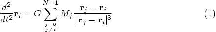
Alice: When we present this to our students, it would be good to summarize
the connection specifically. To wit: the expression for the
acceleration felt by particle i is given by summing together the
Newtonian gravitational attraction of all other particles j, where
both i and j take on values from 1 up to and including N, according
to the text books. In our case, of course, we label particles with numbers
starting from 0 and running up to and including N-1, since that
is Ruby's default way of numbering arrays. Let's write the equations
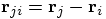
accordingly:
When I write this equation on a black board in front of a class, there
is always someone who asks me where the power of 3 in the denominator
comes from, given that Newtonian gravity is an inverse square law, and
therefore should be proportional to the power 2 of the distance, in
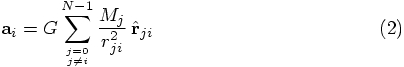
the denominator. To bring out the inverse square nature of gravity,
I then write
Finally, I note that the summation excludes self-interactions: every particle
feels the forces of the other
Bob: That's a nicely crisp summary.
Alice: What is really
nice in our Ruby implementation, is that we never have to introduce
the counters i and j that are so ubiquitous in any N-body code I have
ever seen. Just as we could dispense with the k variable for the
components of a vector, we can avoid the other two counters by asking
arrays and vectors to just loop over themselves.
And this is one of the features that makes Ruby eminently suited
for prototyping and development work in general. Whether Ruby will be used
eventually for an industrial-strength production-type code, that remains
to be seen.
Bob: If so, we'll have to do some very serious speed-up. My impression
so far has been that Ruby is at least a couple orders of magnitude slower
than the equivalent C or Fortran implementation.
Alice: In addition, our leapfrog calculates the acceleration twice
on the Nbody level, and for each particle pair, the relative acceleration
is also computed twice.
Bob: If we had been a little more clever, we would have saved a factor
of four there too. I bet we can speed up our code by a stunning factor of
a thousand or so, if we pull all stops!
Alice: Maybe, we'll see in due time. For now, I think we are being
clever, by not worrying at all about optimization. The point is to bring
out the underlying structure, which is complex enough all by itself. Once
we really see that clearly, we can start optimizing while avoiding confusing
clutter.
Bob: Note, by the way, one more difference between the 2-body and
N-body case: in the latter case we have to accumulate the results,
through the summation you just showed. Before traversing the loop
over particles, we have to clear the vector where the acceleration a
on our particle is being stored. I experimented with various ways to
do so, but the most compact notation I found was what I wrote on the top
of the acc method:
Isn't that a nifty and compact expression?
Alice: I see. In order to provide a null vector for the acceleration
with the right number of components, you use the position as a template,
and after copying the position, you fill all entries with zeroes. I'm
glad you put a comment line in, since otherwise the meaning wouldn't
have been so obvious at first reading.
Hmmm. While I agree that it is compact, perhaps a longer expression would
have been a bit more clear. How about
Alice: Yes, your construction was clever, but I'm still wondering about
the unsuspecting reader, who has to make sense of your cleverness. In fact,
in my more lengthy alternative, notice that I left your comment line
in, since upon first reading, even my longer line would still not be fully
clear, I'm afraid.
If I really wanted to be self-explanatory, I would write:
Bob: A long day, if you ask me. I would never have guessed your explanation
completely just from looking at that piece of code, so I would insert
a comment there as well -- which makes your alternative longer than mine.
I prefer to stick with my
Alice: Fine with me. This is really a matter of taste.
Bob: While we're at it, let me walk you through the rest of the Body
class definition. The potential is constructed in a very similar way
as the acceleration, by doing a body walk through the whole system.
In the two-body case, we started with:
My new N-body version reads:
The difference with respect to acc is that the potential energy
includes a product of the mass of the calling particle i and the
mass of the called particle j:
Bob: The rest of the input and output routines are unchanged, compared to
our earlier two-body code. Let's return to the Nbody class. You mentioned
that the leapfrog method was almost the same as before. Unfortunately,
that is the only one of our four integration methods that remained quite
simple to read. The other three have become a bit more crowded, I'm afraid.
Alice: I'll start with the forward Euler case again. In forward, you
have replaced the previous form
by:
Bob: This is a tricky point. Before we stored the original acceleration
in the vector old_acc, which was a single physical vector, containing
the relative acceleration between our two particles. In the N-dimensional
analogue that we have here, we need to store N initial acceleration vectors,
one for each particle.
The most straightforward solution would be to define a new instance variable
for the Body class, @old_acc, but I rejected that solution.
As you will be happy to hear, I wanted to keep the code modular, without
letting the Body class know what the Nbody class might decide to be
good algorithms. The alternative would be to saddle the poor Body class
simultaneously with all the possible variables that would be needed in all
the algorithms you could choose from.
Alice: I indeed applaud your desire for modularity. However, in this
particular case I'm not so sure whether we should insist on such a strong
separation. Let's get back to that in a moment.
Bob: Since I wanted to keep the auxiliary variables, such as
old_acc, local, I could not loop over them using the
@body.each construct used in leapfrog. Of course, you can
loop over old_acc alone easily enough, in a old_acc.each
construction, but that would in turn not allow the @body array
to be traversed.
The only solution I saw was to introduce an index i -- yes, I know,
we just celebrated the lack of indices i and j in Ruby, and I'm
not happy with it, but at least for now, it works. In that way, I
could use the Array method @body.each_index, which does
what it says it does, namely traversing the @body array.
Now since old_acc and @body have the same number of
components, equal to the number of particles N, this one construct
can simultaneously traverse both arrays. The i index is the glue
that connects both traversals, keeping them in lock step.
In addition, I had to introduce the array old_acc, which I
did here in the first line of forward. The third line did not
contain any local variables, so there at least I could avoid the use
of an i variable.
Alice: That is a reasonable solution. You are trading modularity for
readability. And while I'm sure there are several alternatives, let's
first complete our guided tour here. What is left to visit is the
energy diagnostics part of the code.
Bob: That turned out to be really simple. For each Body method
ekin there is a corresponding Nbody method ekin that gathers all
the individual results, and sums them up to find the total kinetic energy.
Here is the Body version:
and here is the Nbody version:
In order to sum it all up, I introduce a variable e, initialize it to
zero, add the various contributions, and then I list e again, in the
final line. In that way, the method ekin returns the correct value e.
Alice: Just curious: couldn't you have left out the last line, with the
single e? At the last time that the statement in the previous line will
be executed, some particle's kinetic energy will be added to e, so e
will be what is going to be returned anyway, no?
Bob: I'm not sure. You're talking about the last action in a loop, and
then control is being returned to the each method. But it is easy enough
to find out whether that would work. Let's call irb for help:
Bob: Well, I wasn't sure either. Learn something new everyday. And it is
certainly nice to work with an interpreted, rather than a compiled language:
this type of checking you can do extremely quickly and easily.
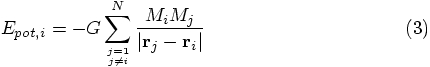
Alice: The story for the potential energy must be similar. For each particle
we have a method epot associated with the Body class, as you just
showed us already, and a method with the same name, but associated
with the Nbody class:
Just like for the kinetic energy, the Nbody method epot gathers
all the contributions to the potential energy of the various bodies --
with one twist: you are now dividing by a factor two. Ah, of course:
for each particle pair, the contribution is counted once when the one
particle computes its potential energy, and once again when the other
particle computes its potential energy. Therefore, every particle pair
contribution gets counted twice, and at the end we have to correct for that.
Bob: Yes, indeed. And yes, I had left that factor of two out, the first
time I ran the program. Diagnostics are wonderful; they sure keep you honest:
of course I could get no good energy conservation no matter what I tried,
until I realized what was going wrong. I found it by computing the initial
kinetic energy and potential energy for a two-body system, which was easy
enough to do on paper. Comparing it with the numerical result, it was
immediately clear that the potential energy was counted twice. 2.1. Inspecting the Leapfrog
   def leapfrog(dt)
     @vel += acc*0.5*dt
     @pos += @vel*dt
     @vel += acc*0.5*dt
   end
2.2. Acceleration
   def acc
     r2 = @pos*@pos
     r3 = r2*sqrt(r2)
     @pos*(-@mass/r3)
   end
2.3. Newtonian Gravity
 and
and  are the mass and position
vector of particle j, and G is the gravitational constant.
are the mass and position
vector of particle j, and G is the gravitational constant.
 , with
  ,
after which I define the unit
vector
,
after which I define the unit
vector 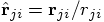 . This allows the
above equation to be written as:
. This allows the
above equation to be written as:
 particles, but not its
own force, which, as we already mentioned, would be infinitely large
in case of a point mass.
particles, but not its
own force, which, as we already mentioned, would be infinitely large
in case of a point mass.
2.4. A Matter of Taste
a = @pos*0 # null vector of the correct length
a = ([0]*@pos.size).to_v # null vector of the correct length
Bob: Yes, that would bring out the fact that you use the position vector
only because you want to extract its size, and not for any other reason.
And you explicitly show how you start with an array of length 1,
filled with a single 0, and then extend that array to contain
@pos.size components. But then you still have to convert it into
a vector. You see, I avoided the last step by starting with a copy of
@pos, which was already a vector.
    vector_size = @pos.size
    a = ([0]*vector_size).to_v
That way I would express the fact that a is a vector, that it needs
to be of the right size, that it should contain all zeroes, and that
it should be converted to a proper vector at the end of the day.
a = @pos*0 # null vector of the correct length
2.5. Potential Energy
   def epot                        # potential energy
     -@mass/sqrt(@pos*@pos)        # per unit of reduced mass
   end
2.6. Local Arrays
   def forward(dt)
     old_acc = acc
     @pos += @vel*dt
     @vel += old_acc*dt
   end
2.7. Energy Diagnostics
   def ekin                        # kinetic energy
     0.5*(@vel*@vel)
   end
   def ekin                        # kinetic energy
     e = 0
     @body.each{|b| e += b.ekin}
     e
   end
  |gravity> irb
  irb(main):001:0> a = [1, 2, 3]
  => [1, 2, 3]
  irb(main):002:0> e = 2
  => 2
  irb(main):003:0> a.each{|b| e += b}
  => [0, 1, 2, 3]
  irb(main):004:0> e
  => 8
Alice: I see. You were correct in worrying about the control coming back
to the array. Actually, that makes sense: it was the array a in
this example that called the each method. And frankly, even if it
would have worked, it might have been better to leave the final e
line in there, at the end of your ekin, for clarity.