18. Leapfrog
Carol: Erica, we now have a second-order algorithm, modified Euler,
but you mentioned an other one, quite a while ago, that you seemed to prefer.
Erica: Yes, the leapfrog algorithm, a nice and simple scheme.
I just learned about that in class, so it is still fresh in my memory.
Dan: What a strange name. Does it let particles jump around like frogs?
Carol: Or like children jumping over each other?
Erica: Something like that, I guess. I never thought about the
meaning of the name, apart from the fact that something is leaping
over something, as we will see in a moment. The algorithm is used
quite widely, although it has different names in different fields of
science. In stellar dynamics you often hear it called leapfrog, but
in molecular dynamics it is generally called the Verlet method, and
I'm sure there must be other names in use in other fields.
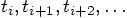
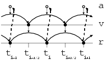
Here is the idea. Positions are defined at times
It is these positions and velocities that `leap over' each other.
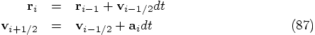
The leapfrog integration scheme reads:
Figure 37: With the leapfrog algorithm, when we update a position value to a new point
in time, we use the information from the velocity value in between the old
and the new point in time. This is indicated by the vertical downward
arrows. Similarly, when we update a velocity value to a new point
in time, we use the information from the acceleration value in between the old
and the new point in time. Each acceleration value is
computed directly from the position value, using Newton's law of gravity.
This is indicated with the dashed upward pointing arrows.
Erica: The simplest way to extrapolate the velocities from
Concretely, we can start with the initial conditions
18.1. Interleaving Positions and Velocities
 , spaced at constant intervals
  , while the velocities are defined at times halfway in
between, indicated by
, while the velocities are defined at times halfway in
between, indicated by 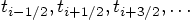 , where
  .
.
 are defined only on
integer times, just like the positions, while the velocities are
defined only on half-integer times. This makes sense, given that the
acceleration on one particle depends only on its position with respect
to all other particles, and not on its or their velocities. To put it
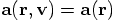
in mathematical terms, for many situations in physics the acceleration
depends on velocity and position, as
are defined only on
integer times, just like the positions, while the velocities are
defined only on half-integer times. This makes sense, given that the
acceleration on one particle depends only on its position with respect
to all other particles, and not on its or their velocities. To put it
in mathematical terms, for many situations in physics the acceleration
depends on velocity and position, as  .
The motion of an electron in a magnetic field is one example, with the
Lorentz force being velocity dependent. And in any situation in which
there is friction, the friction is typically stronger for higher velocities.
However, in the case of Newtonian gravity, the velocity dependence is absent:
.
The motion of an electron in a magnetic field is one example, with the
Lorentz force being velocity dependent. And in any situation in which
there is friction, the friction is typically stronger for higher velocities.
However, in the case of Newtonian gravity, the velocity dependence is absent:
 .
.
 , how are you going to construct the velocities
at time
, how are you going to construct the velocities
at time  ?
?
 to
to  is by using a Taylor series. and the simplest
nontrivial Taylor series is the one that takes only one term beyond the
initial value. It turns out that such utter simplicity is already enough!
is by using a Taylor series. and the simplest
nontrivial Taylor series is the one that takes only one term beyond the
initial value. It turns out that such utter simplicity is already enough!
 and
and  , and take the first term in the Taylor series
expansion to compute the first leap value for
, and take the first term in the Taylor series
expansion to compute the first leap value for  :
:

 ,
using the first leap value for
,
using the first leap value for  .
Next we compute the acceleration
.
Next we compute the acceleration  , using Newton's
law of gravitation, and this enables us to compute the second leap value,
, using Newton's
law of gravitation, and this enables us to compute the second leap value,
 , using the second line of apply
Eq. (87). In this way we just march on.
, using the second line of apply
Eq. (87). In this way we just march on.
Carol: And when you want to stop, or pause in order to do a printout, you can again construct a Taylor series in order to synchronize the positions and velocities, I presume? If you make frequent outputs, you'll have to do a lot of Tayloring around. I wonder whether that doesn't affect accuracy. Can you estimate the errors that will be introduced that way?
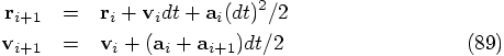
Erica: Ah, the beauty here is: you do not introduce any extra errors! In fact, what we usually do is never use the half-integer values for the velocity in any explicit way. Here, let me rewrite the basic equations of the algorithm, in such a way that position and velocity remain synchronized, both at the beginning and at the end of each step.
Erica: Ha, but looks deceive! Notice that the increment in
Dan: I'm still not quite convinced that Eq. (87) and
Eq. (92) really express the same integration scheme.
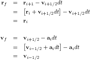
Erica: An interesting way to see the equivalence of the two descriptions
is to note the fact that the first two equations are explicitly
time-reversible, while it is not at all obvious whether the last two
equations are time-reversible. For the two systems to be equivalent,
they'd better share this property. Let us check this, for both cases.
Carol: Eq. (87) indeed looks pretty time symmetric.
Whether you jump forward or backward, in both cases you use the same
middle point to jump over. So when you first jump forward and then
jump backward, you come back to the same point.
Erica: Yes, but I would like to prove that, too, in a mathematical
way. It is all too easy to fool yourself with purely language-based
analogies.
Dan: Spoke the true scientist!
Carol: Well, I agree. In computer science too, intuition can lead you
astray quite easily. How do you want to check this?
Erica: Let us first take one step forward, taking a time step
We now have to inspect where the final positions and velocities
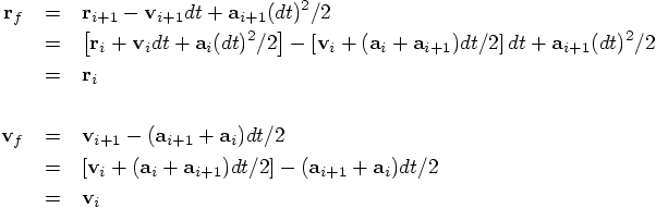
Don: Amazing indeed, but I would be really amazed if the same time
symmetry would hold for that other set of equations,
Eq. (92), that don't look time symmetric at all!
Erica: Yes, that's where the real fun comes in. The derivation
is a bit longer, but equally straightforward, and the steps are all
the same. Here it is:
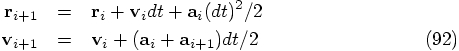
Dan: Okay, I'm convinced now that Eq. (92) does the
right thing. Let's code it up, and for convenience, let me write down
the equations again:
Let me see whether I'm getting the hang of using vectors now.
I will put it in file leapfrog_try1.rb:
and let me make a picture right away, in figure 38:
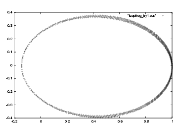
Figure 38: First attempt at leapfrog integration, with step size
Erica: That is in fact an essential part of the leapfrog algorithm.
If it would drift in one direction, and if you would then play time
backward, it would have to drift in the other direction -- which means
it would not be time symmetric. So because the leapfrog is time
symmetric, it is impossible for the orbits to drift!
Dan: Ah, I just noticed something. In my leapfrog implementation,
I compute the acceleration at the end of the loop, and then at the
beginning of the next loop, I calculate the exact same acceleration
once again. Since the position r does not change between the two
calculations, the value of the acceleration a is bound to be the
same. That's a waste of computing time!
Carol: Well, for the two-body problem, we don't have to worry too much
about exactly how many milliseconds of computer time we are spending.
Erica: True, but when we go to a thousand-body problem, this will become
an issue. Good point, Dan, why don't you leave one of the acceleration
calculations out from the loop.
Dan: The question is, which one. If I leave out the first one,
the acceleration is not yet defined, when the loop gets transversed
for the very first time. But if I leave out the second one, I cannot
calculate the value of the velocity at the end of the loop.
Hmmm. The second acceleration calculation is clearly essential.
But . . . , aha, I see! I can take out the first acceleration calculation
and place it before the loop. That way, the length of the computer
program does not change. However, inside the loop unnecessary
calculations are no longer being done.
Here is the new version, in file leapfrog_try2.rb:
Let me check first to see that we get the same result. The first
code gives:
Carol: Let's check whether you really made the computation faster.
We can redirect the standard output to /dev/null, literally
a null device, effectively a waste basket, which is a Unix way of
throwing the results away. That way, we are left only with output
that appears on the standard error channel, such as timing information
provided by the time command.
The first code gives:
Carol: But we can make it even more clear, and we can make the loop
even shorter, with the help of our old friend, the DRY principle. Look,
the calculation for the acceleration, before and in the loop, contains
the exact same three lines. Those lines really ask to be encapsulated
in a method. Let me do that, in file leapfrog.rb:
and as always, I'll test it:
 is given by the time step multiplied by
 , effectively equal
to
, effectively equal
to  . Similarly, the increment in
 is given by the time step multiplied by
 , effectively equal to the
intermediate value
, effectively equal to the
intermediate value  . In conclusion,
although both positions and velocities are defined at integer times,
their increments are governed by quantities approximately defined at
half-integer values of time.
. In conclusion,
although both positions and velocities are defined at integer times,
their increments are governed by quantities approximately defined at
half-integer values of time.
18.2. Time Symmetry
 , to evolve
  to
to
 . We can then take one
step backward, using the same scheme, taking a time step of
. We can then take one
step backward, using the same scheme, taking a time step of
 , back in time. Clearly, after these two steps the
time will return to the same value since
, back in time. Clearly, after these two steps the
time will return to the same value since 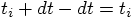 .
.
 are indeed equal to
their initial values
are indeed equal to
their initial values 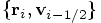 . Here is
the calculation. First we apply the first line of Eq. (87)
to compute
. Here is
the calculation. First we apply the first line of Eq. (87)
to compute  as the result of the step back in time,
and then we again apply the first line of Eq. (87), to
compute the forward step, and we see that indeed
as the result of the step back in time,
and then we again apply the first line of Eq. (87), to
compute the forward step, and we see that indeed
 . Next we apply the second line of
Eq. (87) two times, to find that
. Next we apply the second line of
Eq. (87) two times, to find that
 . Here is the whole derivation:
18.3. A Vector Implementation
 to time
  , with both positions and
velocities.
, with both positions and
velocities.
|gravity> ruby leapfrog_try1.rb > leapfrog_try1.out
 .
.
18.4. Saving Some Work
 |gravity> ruby leapfrog_try1.rb | tail -1
 0.583527377458303  -0.387366076048216  0.0  1.03799194001953  0.167802127213742  0.0
and the second version gives:
 |gravity> ruby leapfrog_try2.rb | tail -1
 0.583527377458303  -0.387366076048216  0.0  1.03799194001953  0.167802127213742  0.0
Good.
 |gravity> time ruby leapfrog_try1.rb > /dev/null
 0.352u 0.001s 0:00.38 92.1%    0+0k 0+0io 0pf+0w
and the second version gives:
 |gravity> time ruby leapfrog_try2.rb > /dev/null
 0.194u 0.000s 0:00.21 90.4%    0+0k 0+0io 0pf+0w
Dan: Indeed, a bit faster. If all the computer time would have
been spend on acceleration calculation, things would have sped up
by a factor two, but of course, that is not the case, so the speed
increase should be quite a bit less. This looks quite reasonable.
18.5. The DRY Principle Once Again
 |gravity> ruby leapfrog.rb | tail -1
 0.583527377458303  -0.387366076048216  0.0  1.03799194001953  0.167802127213742  0.0